Transcoders: Interpretable MLP Replacements

The MLP Problem

Every transformer layer has two main components: attention heads that move information between positions, and MLPs that apply nonlinear transformations at each position. The QK and OV decomposition gives us useful tools for analyzing how attention heads select and move information. MLPs are harder to decompose because their transformations are dense and nonlinear.

Sparse autoencoders offered a partial solution. By training an SAE on a layer's activations, we can decompose those activations into sparse, interpretable features. But SAEs reconstruct the same activation they receive as input. They reveal what features are present at a given layer, not how information transforms as it passes through the MLP. An SAE placed at the MLP output tells us what features exist after the MLP computation. It does not tell us which input features produced which output features.The distinction is subtle but important. An SAE asks: 'What features are encoded in this activation vector?' A transcoder asks: 'What function does this MLP compute, expressed in terms of sparse features?' The first is a question about representation; the second is a question about computation.

For circuit analysis, we need to trace causal paths through MLP layers, not just observe what comes out the other side. This is what transcoders provide.

What Is a Transcoder?

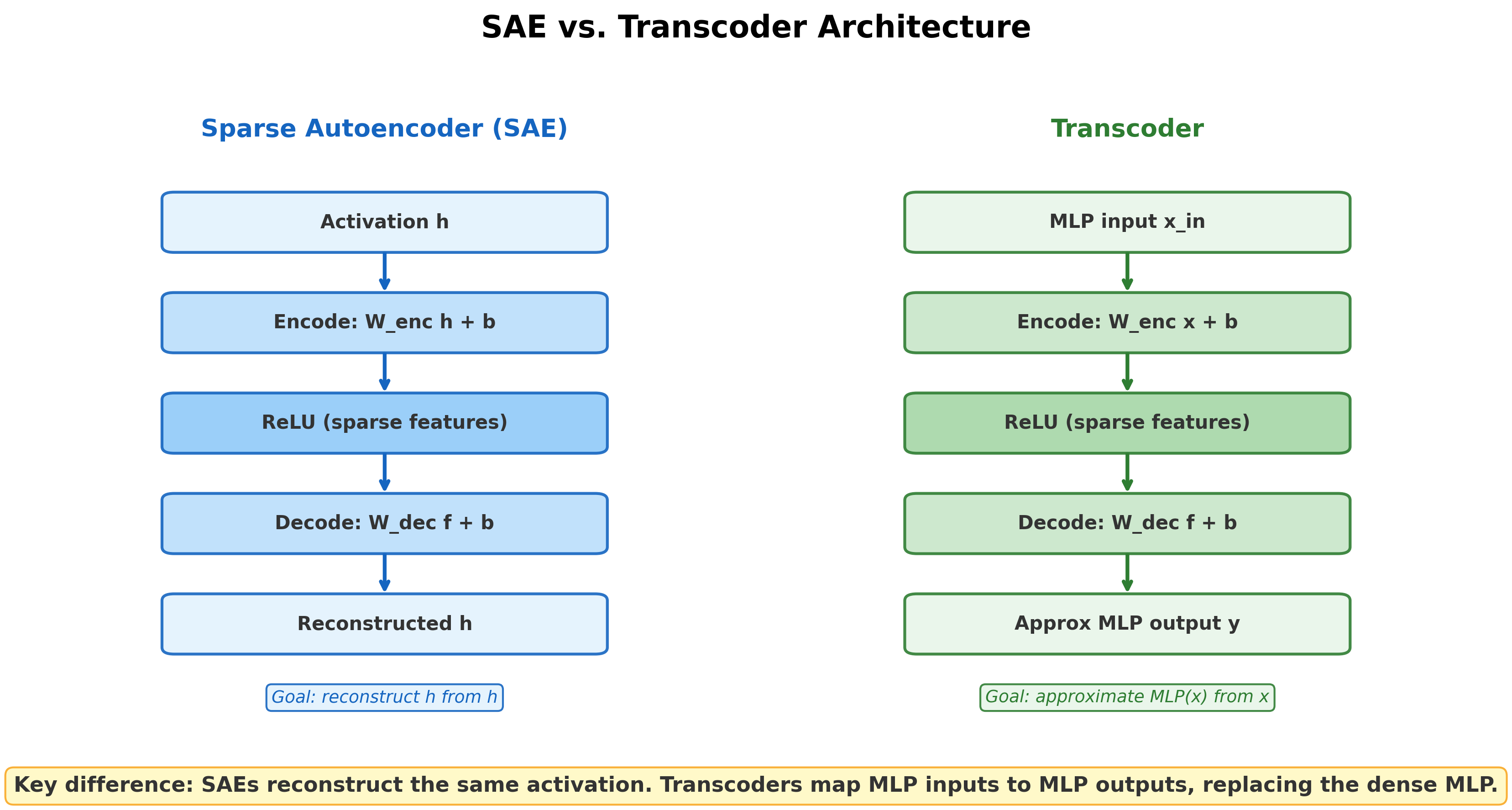
Transcoder: A transcoder is a modified sparse autoencoder that approximates MLP behavior. Instead of encoding and reconstructing the same activation, a transcoder takes the MLP input $\mathbf{x}_{\text{in}}$ and produces an approximation of the MLP output $\mathbf{y}_{\text{out}}$:

$$\mathbf{y}_{\text{out}} \approx \text{ReLU}(\mathbf{x}_{\text{in}} W_{\text{enc}} + \mathbf{b}_{\text{enc}}) W_{\text{dec}} + \mathbf{b}_{\text{dec}}$$

The transcoder replaces the dense MLP with a wider, sparsely-activating layer.

The architecture has the same broad parts as an SAE: an encoder, a sparse bottleneck, and a decoder. The input and output differ, however. An SAE maps $\mathbf{h} \to \mathbf{h}$. A transcoder maps $\mathbf{x}_{\text{in}} \to \mathbf{y}_{\text{out}}$, where $\mathbf{x}_{\text{in}}$ enters the MLP and $\mathbf{y}_{\text{out}}$ is the output the MLP would produce. The transcoder approximates the MLP's function rather than reconstructing one representation.

From Sparse Replacement to Circuit Node

Sparse autoencoders (SAEs) decompose representations, whereas transcoders decompose computations:

SAEs decompose what a layer represents. Given activation $\mathbf{h}$, an SAE finds sparse features $\mathbf{f}$ such that $\mathbf{h} \approx \mathbf{f} W_{\text{dec}}$. This is useful for understanding individual layers but does not reveal how features at one layer produce features at the next.

Transcoders decompose what a layer computes. Given MLP input $\mathbf{x}_{\text{in}}$, a transcoder finds sparse features that produce the MLP output. Because the transcoder's features map inputs to outputs, we can trace how upstream features contribute to downstream features through the MLP.In the residual stream picture, attention heads move information between positions while MLPs transform information at each position. SAEs decompose the residual stream at a point. Transcoders decompose the transformation that happens between points. Both are needed for complete circuit analysis.

The input-output map lets us trace attributed paths through MLP layers rather than treating each MLP as a black box. The claim remains about the transcoder replacement until interventions confirm that the corresponding pathway matters in the original model.

Clean Factorization

Dunefsky et al. (2024) showed that transcoder circuits factorize cleanly into two terms [1]Transcoders Find Interpretable LLM Feature Circuits
Dunefsky, J., Chlenski, P., Nanda, N.
NeurIPS, 2024:

• An input-dependent term: which transcoder features activate on this particular input
• An input-invariant term: how feature activations map to outputs through the decoder weights

This factorization supports weight-based analysis through an MLP replacement. The decoder gives each transcoder latent a fixed output direction, while the encoder determines which latents fire on an input. The account remains approximate because the transcoder does not reproduce the original MLP perfectly and its learned latents may not be uniquely determined.

Dunefsky et al. applied transcoders to GPT-2 Small's greater-than circuit, the circuit that processes prompts like "The war started in 1742 and ended in 17__". Transcoders revealed sub-computations within the circuit that were invisible at the head level, showing that the circuit was more modular than previously understood.

Pause and think: SAEs vs. transcoders

SAEs reconstruct the same activation they receive. Transcoders map MLP inputs to MLP outputs. Why does this difference matter for tracing how information flows through a network?

Think about what it means to follow a causal chain from input to output. Attention exposes an explicit routing pattern and a linear value-to-output map once that pattern is fixed; an MLP applies a dense nonlinear map at one position. An SAE at the MLP output describes candidate features after the transformation but does not model the input-output map. A transcoder supplies a sparse approximation of that map, letting an attribution method propose paths through the replacement rather than skipping the MLP entirely.

Transcoders vs. SAEs: A Direct Comparison

Paulo et al. (2025) compared transcoders and SAEs trained on the same model and data:

• On the study's automated and human-scored evaluations, transcoder features scored as more interpretable than the matched SAE features.
• Skip transcoders, which add an affine skip connection, achieved lower reconstruction loss without a measured interpretability reduction in this comparison.
• Transcoders also improved several tested SAEBench tasks, including feature-absorption and sparse-probing evaluations.

The comparison gives transcoders a structural advantage for questions about what an MLP maps from input to output. SAEs remain suited to describing features present at one activation site, while either method can inherit dictionary non-uniqueness and reconstruction error.A benchmark win does not make transcoders a universal replacement for SAEs. The choice depends on whether the object of interest is a representation at one site or a transformation between two sites.

From Transcoders to Circuit Tracing

Transcoders address a specific problem: exposing an approximation of an MLP's computation. Combined with attention analysis, they let researchers trace feature-level paths through both kinds of transformer sublayer.

Marks et al. [2]Sparse Feature Circuits: Discovering and Editing Interpretable Causal Graphs in Language Models
Marks, S., Rager, C., Michaud, E. J., et al.
ICLR 2025, 2024 demonstrated that SAE features can serve as the nodes in causal circuit graphs, sparse feature circuits. This was an important step, but the approach still relied on per-layer SAEs and computationally expensive patching.

Lindsey et al. [3]Circuit Tracing: Revealing Computational Graphs in Language Models
Lindsey, J., Batson, J., Denison, C., et al.
Anthropic, 2025 build attribution graphs by replacing MLPs with cross-layer transcoders and tracing selected effects backward through the feature network with Jacobian-based attribution. The resulting graph is a sparse, input-specific approximation, not a complete map of every computation used by the original model.

The methods form a progression in resolution: transcoders approximate an MLP with sparse latents, sparse feature circuits use learned features as graph nodes, and attribution graphs combine replacement models with scalable edge attribution. Circuit Tracing and Attribution Graphs covers the resulting evidence and its limits.

Pause and think: What changes with feature-level circuits?

In the IOI circuit analysis, the circuit had 26 attention heads as nodes. With transcoders enabling feature-level analysis, circuits can have thousands of feature nodes. What do we gain from this higher resolution? What do we lose?

We gain a more granular hypothesis for each node, and we can trace through MLPs instead of treating them as gaps. We lose simplicity: a 26-node circuit diagram can be inspected directly, while a 2,000-node feature graph requires pruning, automated tools, and checks that important paths were not omitted.

Looking Ahead

Sparse autoencoders describe what is present at one activation site; transcoders approximate the map from one site to another. That input-output factorization makes multilayer perceptrons easier to include in a circuit, but the circuit describes the replacement only as faithfully as the transcoder reconstructs the original computation.

Circuit Tracing and Attribution Graphs builds on cross-layer transcoders to trace input-specific effects through thousands of features, then examines how approximation error, frozen attention, and local attribution limit the resulting graphs.