The Residual Stream as a Vector Space
The residual stream is more than just a convenient name. It is a -dimensional vector that lives in , and treating it as a proper vector space unlocks the mathematical framework behind mechanistic interpretability [1]A Mathematical Framework for Transformer Circuits
Elhage, N., Nanda, N., Olsson, C., et al.
Anthropic, 2021.
If you want a refresher on prerequisites or a full architecture walkthrough, start with Prerequisites and Transformer Architecture Intro.
At each token position, the residual stream starts as the token embedding and accumulates additive updates from every attention head and MLP layer. The final residual stream at any position decomposes as a sum:
Each term in this sum is a vector in . Every component reads the current residual stream and writes an update back to it.Components can favor different read and write subspaces. Orthogonal direct subspaces do not interact through a simple dot product, but normalization and later components can still couple their effects. Additivity makes bookkeeping possible; it does not make the full computation independent.
Residual Stream (Formal): The residual stream is the -dimensional vector that flows through the transformer, starting as the token embedding and accumulating additive updates from each attention head and MLP layer.
The additive residual stream lets us isolate a component's direct contribution and ask how it affected a prediction. Later components can transform or compensate for that update, so studying terms separately is a useful starting point rather than a complete account of causality.
Two Jobs, One Head
Each attention head does two conceptually independent things. First, it decides where to move information: which source tokens should each destination token attend to? Second, it decides what information to move: given the attended tokens, what gets copied to the output?
These two jobs are controlled by two parameter products: the QK circuit and the OV circuit. The four weight matrices of an attention head (, , , ) factor into these two products, which can be inspected separately while remembering that the head's behavior also depends on its inputs.
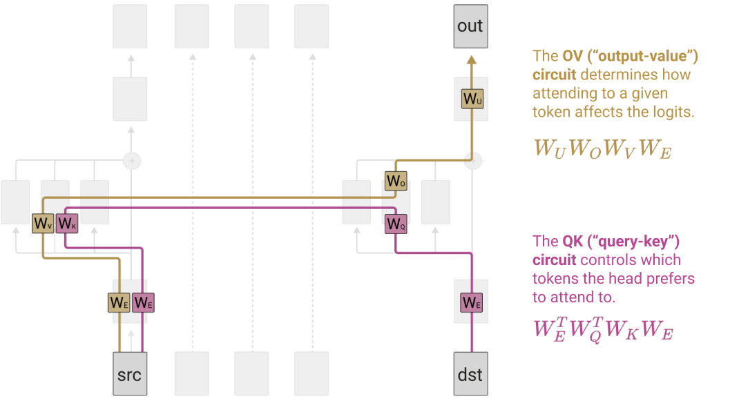
Elhage, N., Nanda, N., Olsson, C., et al.
Anthropic, 2021
The QK Circuit
QK Circuit: The QK circuit of attention head is the matrix . It determines the attention pattern: which source tokens each destination token attends to.
The attention score between tokens and can be written directly in terms of the QK circuit:
where and are the residual stream vectors at positions and . This is a bilinear form on : it takes two residual stream vectors and produces a scalar score. No separate query and key vectors need to be computed; the QK circuit matrix directly answers "how much should token attend to token ?"The QK circuit is a matrix, but it has rank at most because it is the product of a matrix with a matrix. This low-rank structure means each head can only compute attention scores using a -dimensional subspace of the residual stream.
We can go further. Including the embedding and unembedding matrices, the full end-to-end QK circuit maps tokens to attention scores:
This is an matrix. Entry tells us "how much does token attend to token , based purely on token identity?" This is a directly interpretable object: a token-to-token attention score matrix that we can inspect.
The OV Circuit
OV Circuit: The OV circuit of attention head is the matrix . It determines what information is moved from attended-to tokens to the destination.
The output contribution from source token to destination token is:
where is the attention weight. The OV circuit is a single matrix that transforms each source token's information before writing it to the residual stream. Like the QK circuit, it has rank at most , creating a low-rank bottleneck that forces the head to compress its processing into a limited-dimensional subspace.
The full end-to-end OV circuit, including the unembedding, is:
This is also an matrix. Entry tells us "if the head attends to token , how much does that increase the logit for token ?" This directly reveals the effect on predictions of attending to a given token.
QK vs. OV: Side by Side
The two circuits have complementary roles:
| QK Circuit (Where to Look) | OV Circuit (What to Move) | |
|---|---|---|
| Matrix | ||
| Input | Two token positions | A source token |
| Output | An attention score | An update to the residual stream |
| Answers | "Should I attend here?" | "What should I copy?" |
| End-to-end | ||
| Interpretation | Token-to-token relevance | Token-to-logit effect |
Every attention head decomposes into these two circuits. This is more than compact notation: it separates where the head looks from what it moves. The two parameter products are independent, although their effects inside a full model still interact with the residual stream, normalization, and later layers.
Pause and think: Why independence matters
Consider an attention head that always attends to the previous token (a "previous token head"). Its QK circuit determines where it looks (always one position back). Its OV circuit determines what it copies from that position. You could change what the head copies without changing where it looks, or vice versa. Why is this independence important for mechanistic interpretability? What would it mean if the two circuits were entangled instead?
A Worked Example
To make the QK/OV decomposition concrete, consider a tiny 1-layer, attention-only transformer with , one attention head, and no MLP or layer norm. We trace a 2-token input through the standard computation, then verify that the circuit view gives identical results.
Setup. Embedding vectors and . Weight matrices: (identity), is a permutation that swaps entry pairs and , is a permutation that swaps entries 2 and 3, and .
Standard computation. Since , the queries equal the embeddings: and . For the keys, swaps pairs: and .
The raw attention scores for token A are and . Scaling by gives and , and softmax yields and . Token A pays 92% of its attention to token B.
The values are and (after swaps entries 2 and 3). The attention output for token A is .The output is dominated by because A attends mostly to B. The QK circuit determined where A should look (at B), and the OV circuit determined what gets copied (B's value vector, transformed by ).
The QK circuit view. The QK circuit matrix is . Since is a symmetric permutation, . Computing the attention score directly:
Same answer as the standard computation, in a single matrix multiplication.
The OV circuit view. The OV circuit matrix is . The output from attending to token B is , matching exactly.
The takeaway. The standard four-matrix view (, , , ) and the two-circuit view (, ) produce identical results. But the circuit view reveals the structure: the QK circuit is a single matrix that directly gives attention scores, and the OV circuit is a single matrix that directly gives the output transformation. Each head has exactly two independent functions, and we can study them separately.
Pause and think: Extending the example
In this toy example, and were identity matrices for simplicity. In a real transformer, all four weight matrices are learned. How would the QK and OV circuits change if were not the identity? Would the independence of the two circuits still hold? Think about what conditions are needed for the QK circuit to be truly independent from the OV circuit.
The One-Layer Model
For a one-layer, attention-only model, the full output has a clean closed form:
where is the attention pattern matrix produced by the QK circuit and softmax. The model output is the original token embedding plus a sum of OV-circuit outputs, weighted by the attention patterns. Every part of this expression is inspectable: tells us where each head looked, and tells us what it moved.This clean decomposition is why one-layer and two-layer attention-only transformers are the starting point for much of the mathematical framework in Elhage et al. (2021). The absence of MLPs and the limited depth make it possible to write the full computation as a sum of interpretable terms.
This decomposition is the foundation for the composition framework covered in the next article. When we stack multiple layers, layer 2 heads can read the outputs of layer 1 heads from the residual stream, creating composed behaviors that neither head could achieve alone.
From Token Space to Feature Space
The QK/OV decomposition provides the vocabulary researchers use to describe what attention heads do. Calling a head a "previous token head" or an "induction head" makes two claims: its QK circuit selects a particular source, and its OV circuit writes a particular effect. The framework from Elhage et al. [3]A Mathematical Framework for Transformer Circuits
Elhage, N., Nanda, N., Olsson, C., et al.
Anthropic, 2021 turns four opaque weight matrices into two objects with distinct functional roles.
The mathematical framework also gives us concrete, inspectable matrices. The end-to-end QK circuit is a vocabulary-sized matrix we can examine entry by entry. The end-to-end OV circuit directly tells us how attending to each token affects the output logits. These are not abstractions; they are real, computable objects that researchers use every day to understand what transformers learn.
The token-to-token view is most direct in shallow models where the residual stream is close to the token embeddings. In deeper models, each position contains a mixture of learned features. Circuit Tracing develops QK attribution, which expands those residual streams into sparse features and decomposes an observed attention score into query-feature and key-feature interactions.