Circuits in Parameter Space

Why Attention Resists Decomposition

Circuit tracing lists frozen attention as a standing limitation: attribution graphs hold the attention patterns fixed and report first-order effects through them [1]Circuit Tracing: Revealing Computational Graphs in Language Models
Lindsey, J., Batson, J., Denison, C., et al.
Anthropic, 2025. The reason is structural rather than incidental. A transcoder replaces an MLP, a map from one activation to another. An attention score is not that shape: it is bilinear in the activations at two different positions. Several activation-based decompositions of attention have been proposed, and Bushnaq et al. judge that none is yet satisfactory [2]Interpreting Language Model Parameters
Bushnaq, L., Braun, D., Clive-Griffin, O., Bussmann, B., Hu, N., Ivanitskiy, M., Linsefors, L., Sharkey, L.
Goodfire, 2026.

Attention heads are the standard way to carve up an attention layer, but a single computation can be spread across several of them, so a head is not guaranteed to be one thing either.

Parameter subcomponents are vectors in parameter space, and $W_Q$, $W_K$, $W_V$, and $W_O$ are stored concatenated across heads, so a subcomponent spans all the heads in its layer by default. Whether it uses them is an empirical question, and we can check by splitting each subcomponent's weights per head and measuring the norm in each.

Everything below comes from one decomposition: adVersarial Parameter Decomposition (VPD) applied to a four-layer 67M-parameter transformer trained on the Pile [3]Interpreting Language Model Parameters
Bushnaq, L., Braun, D., Clive-Griffin, O., Bussmann, B., Hu, N., Ivanitskiy, M., Linsefors, L., Sharkey, L.
Goodfire, 2026. In its layer 1, most $W_Q$ and $W_K$ subcomponents carry nonzero norm in all six heads, and none is exclusively localized to one. The $W_V$ and $W_O$ subcomponents look similar.

Nonzero weights are not the same as used weights, so this is suggestive rather than conclusive. Settling it means seeing what the subcomponents compute.

The QK Circuit as Pairs of Subcomponents

Recall the QK circuit of head $h$, the matrix $W_{QK}^h = W_Q^h (W_K^h)^T$ that turns a pair of residual-stream vectors into an attention score, $e_{i,j} = \mathbf{x}_i \, W_{QK}^h \, \mathbf{x}_j^T$.

Substituting the rank-one decompositions of the query and key matrices, $W_Q^h = \sum_c \mathbf{v}_{Q,c}^T \mathbf{u}_{Q,c}^h$ and $W_K^h = \sum_{c'} \mathbf{v}_{K,c'}^T \mathbf{u}_{K,c'}^h$:

$$W_{QK}^h = \sum_{c, c'} \big( \mathbf{u}_{Q,c}^h \cdot \mathbf{u}_{K,c'}^h \big) \, \mathbf{v}_{Q,c}^T \, \mathbf{v}_{K,c'}$$

The decomposition of $W_Q$ and $W_K$ was, without anyone asking for it, also a decomposition of the QK circuit. Pushing the residual-stream vectors through:

$$e_{i,j} = \sum_{c, c'} \big( \mathbf{u}_{Q,c}^h \cdot \mathbf{u}_{K,c'}^h \big) \, ( \mathbf{x}_i \cdot \mathbf{v}_{Q,c} ) \, ( \mathbf{x}_j \cdot \mathbf{v}_{K,c'} )$$

Every attention score is a sum over pairs of subcomponents, one term per pair, and each term is a product of three scalars. Two of them depend on the data: $\mathbf{x}_i \cdot \mathbf{v}_{Q,c}$ asks how strongly the destination token matches what query subcomponent $c$ reads for, and $\mathbf{x}_j \cdot \mathbf{v}_{K,c'}$ asks the same of the source token and key subcomponent $c'$. The third, $\mathbf{u}_{Q,c}^h \cdot \mathbf{u}_{K,c'}^h$, is fixed by the weights.

That third term is what it means for two subcomponents to interact. Recall that each one writes into the head's $d_{\text{head}}$-dimensional query-key space, and the attention score is a dot product taken in that space. If the two write directions point the same way, then a destination token matching $c$ and a source token matching $c'$ together push the score up. If the write directions are orthogonal, the pair contributes nothing regardless of which tokens are present. A strongly interacting pair is therefore a rule of the form destination tokens with property $c$ attend to source tokens with property $c'$, and a head's attention pattern is the sum of however many such rules happen to be active.

Comparing these couplings across pairs takes one correction, because the factorization has a scale degeneracy: multiplying $\mathbf{u}$ by $\lambda$ and dividing $\mathbf{v}$ by $\lambda$ leaves the rank-one matrix $\mathbf{v}^T \mathbf{u}$ untouched. The norm of $\mathbf{u}$ on its own is therefore arbitrary, and only the product $\lVert \mathbf{u} \rVert \lVert \mathbf{v} \rVert$ is pinned down by the decomposition. Scaling each $\mathbf{u}$ by the norm of its partner $\mathbf{v}$ cancels the degeneracy and gives a quantity that can be compared between pairs: the static interaction strength.

Rotary position embeddings rotate queries and keys by an amount that depends on their separation, so in a model that uses them the QK circuit is not one matrix but a family indexed by the offset $\tau$ between the two positions [4]Interpreting Language Model Parameters
Bushnaq, L., Braun, D., Clive-Griffin, O., Bussmann, B., Hu, N., Ivanitskiy, M., Linsefors, L., Sharkey, L.
Goodfire, 2026. Static interaction strength is accordingly a curve over offsets rather than a single number: a pair can couple strongly at short range and weakly at long range, or the reverse. That curve is a readable description of what the rule does.

One Rule, Shared by Five Heads

In the 67M model Bushnaq et al. decompose, layer 1 head 1 is the canonical previous-token head, placing about 60% of its attention on the immediately preceding position. It is not the only head doing so. Four of the other five in that layer also put substantial attention on the last few tokens, just less of it.

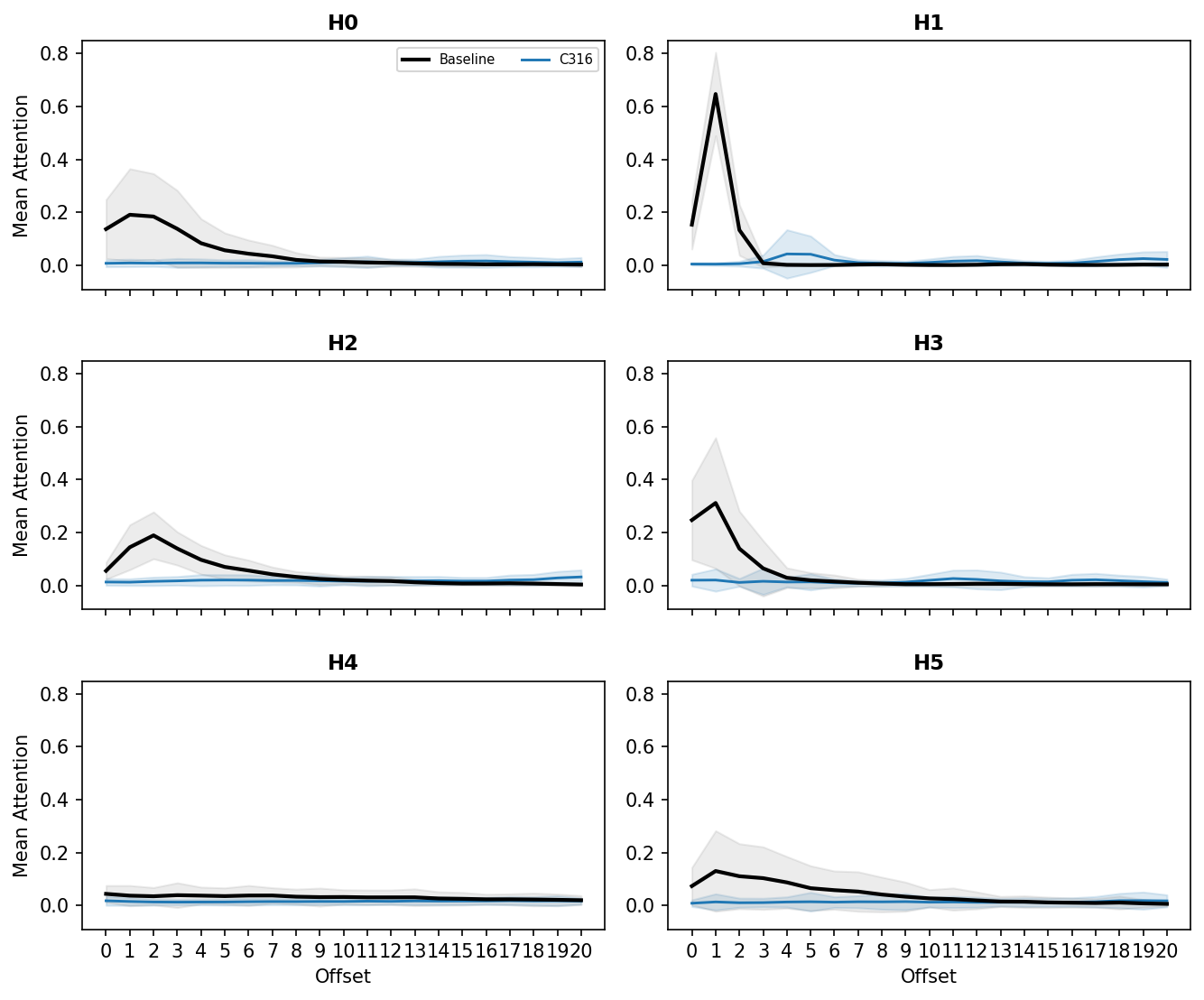
Two subcomponents in layer 1 stand out for being both the largest in norm and the most frequently causally important: a query subcomponent (316) active on 96.7% of tokens and a key subcomponent (329) active on 99.8%. Both carry their largest norm in L1H1 and substantial norm in the other heads. Their static interaction strength is strongly positive at small offsets and weak or negative at distant ones, which is the signature of a rule that says "attend to what just happened."

Ablating subcomponent 316 and re-measuring the attention patterns tests this directly.

Attention to recent offsets collapses in every head that had it, and ablating any other query subcomponent changes nothing distinguishable from baseline. So the recent-token attention in all five heads runs through one rank-one piece of $W_Q$ paired with one rank-one piece of $W_K$. This is a single rule, and the five heads share it rather than each maintaining a copy.

Their OV circuits read from noticeably different subspaces of the residual stream, which the authors offer as weak evidence that the heads gather different information rather than duplicating each other's work.

The Same Query, a Different Key

Sixty percent of L1H1's attention goes to the previous token. Pairing the same query subcomponent with a different key exposes part of what the rest is doing.

Key subcomponent 119 fires on brackets, punctuation, newlines, LaTeX dollar signs and end-of-text tokens, on 16% of tokens. Paired with query 316 the offset dependence inverts: the coupling is strongest at distant offsets. The two together route attention back to the last syntactic boundary, which is the bookkeeping a code model needs constantly -- whether a bracket is still open, whether we are inside a quotation.

Query 316 fires on almost every token, so its side of the rule is always asking; key 119 fires rarely, so it decides which source positions can answer. The two sides are doing different jobs. And again no head owns the rule: nearly every head in the layer shows the interaction, differing only in how far back it reaches.

Pause and think: what would head-level analysis have concluded?

Suppose we only had head-level tools: attention pattern inspection, head ablation, path patching. Looking at L1H1 we would find strong previous-token attention plus a weaker tendency to attend to punctuation, and we would probably call the head polysemantic and move on. Looking at L1H4 we would find long-range attention to punctuation and call it something else entirely.

Both descriptions are true and both are the wrong cut. The actual objects are two query-key subcomponent pairs sharing a query, each spread across most of the layer's six heads, with the heads differing in how far back they apply the rule. Neither the individual head nor the individual pair is visible from the other level.

This is what "attention head superposition" means concretely, and it is why the unit of analysis question in the previous article is not merely philosophical.

Attribution Graphs Over Subcomponents

Individual subcomponents, and interactions within one attention layer, are not yet an account of how a model gets from input to output. For that we need to trace across layers, which means attribution graphs again -- with subcomponents as nodes.

The edges are gradients, but not the plain partial derivative. The derivative $\partial a_c / \partial a_{c'}$ between two subcomponent activations mixes direct influence with influence routed through intermediate subcomponents, and in a residual network the direct path can skip many layers. So gradients are stopped at every subcomponent other than the source, isolating the direct effect, and the derivative is multiplied by the source's activation and its causal importance:

$$\text{attr}(c' \to c) = \left( \frac{\partial a_c}{\partial a_{c'}} \right)^{*} \cdot a_{c'} \cdot g_{c'}$$

The asterisk marks the stopped gradients. Multiplying by $g_{c'}$ keeps causally unimportant subcomponents out of the graph.

Even simple prompts activate hundreds of subcomponents, so graphs get pruned to the ones that matter for one prediction at one position.

Pruning Without an Adversary Finds Circuits That Are Too Small

Pruning means re-optimizing causal importances to be minimal subject to still predicting the target token. There are two ways to do it, and on the same prompt they return graphs of very different sizes.

Prune with stochastic and adversarial mask sampling, as in the decomposition training itself, and the graph for predicting ·her in "The princess lost her crown." keeps 150 subcomponents. Prune with causal importances alone -- no sampling, just minimize the masks while holding the loss down -- and the graph is far smaller and looks considerably more interpretable.

Without robustness to adversarial ablation, the optimization is free to mark subcomponents unimportant that the model actually needs, because nothing ever tests them in combination. The smaller graph is not a coarser summary of the larger one; it claims a simple mechanism where a more complicated one exists. Naively pruned graphs often score better on the task than the target model does, reaching near 100% accuracy on a prediction the real model assigns 0.586.

Predicting the closing > in <u,v depends on layer 1's attention output subcomponents: ablate them from the target model and the probability of > falls from 0.547 to 0.015. Ablate them from the adversarially pruned graph and it falls to 0.021, tracking the real model. Ablate them under causal-importance masking alone and it stays at approximately 1.000, so the naive graph reports that removing something essential changes nothing.

Masking without adversarial sampling is how a large fraction of the subgraph-identification literature finds important subnetworks in large causal graphs, and the problem should apply wherever it is used [6]Interpreting Language Model Parameters
Bushnaq, L., Braun, D., Clive-Griffin, O., Bussmann, B., Hu, N., Ivanitskiy, M., Linsefors, L., Sharkey, L.
Goodfire, 2026. Methods that select a subnetwork by optimizing a differentiable mask over components are hit most directly. But the underlying issue is more general, because the standard automated circuit-discovery methods also never test the excluded components in combination: ACDC removes edges along one greedy trajectory, checking a single ablation configuration at each step [7]Towards Automated Circuit Discovery for Mechanistic Interpretability
Conmy, A., Mavor-Parker, A. N., Lynch, A., et al.
NeurIPS, 2023, and attribution-based edge pruning estimates each edge's effect linearly [8]Attribution Patching Outperforms Automated Circuit Discovery
Syed, A., Rager, C., Conmy, A.
BlackboxNLP 2024, 2023. Neither ever asks whether some other combination of the discarded edges would have broken the model. If the argument holds, published circuits found this way are systematically smaller than the mechanisms they claim to describe, and circuit evaluation needs a stricter bar than the ones currently in use.

The ·her graph raises the probability of the correct token to 1.000 under causal-importance masking and 0.999 under stochastic masking, but only to 0.443 under adversarial masking, below the target model's own 0.586. Even the adversarially pruned graph is leaving relevant computation out.

The <u,v graph keeps 158 subcomponents, most of them specialized for closing delimiters or for angle brackets in particular. Tracing it backward shows the information about the opening < reaching the final position through layer 1 attention by both of the routes from earlier in this article: the previous-token pair carries it forward in time, and the syntax-boundary pair carries it as formatting information. Two rules studied separately turn out to be parts of one prediction.

Editing One Rank-One Piece

Because the decomposition stays inside the original architecture, its pieces are weights, so editing a piece edits the model. No transcoder can offer that.

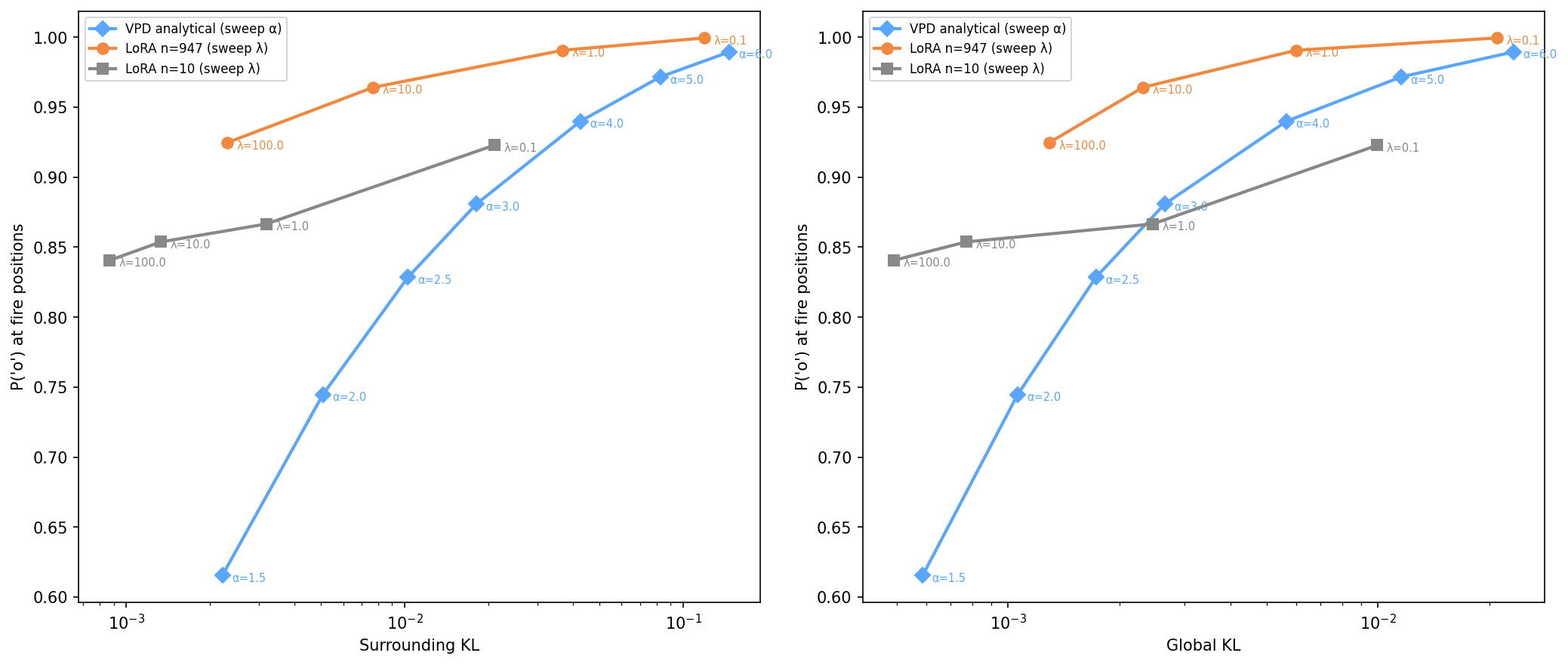
The target here is deliberately small. The model should predict that every emoticon is a surprised face, :o, and nothing else should change. A token-level remap cannot do it, because :, ;, X and = appear constantly outside emoticons, so any rule keyed on the token is wrong most of the time. The edit has to be conditioned on the model's own judgment that an emoticon is underway, which means editing the mechanism that makes that judgment. Six subcomponents in layer 2's MLP down-projection are candidates: they fire on emoticon-initial characters and stay quiet on those same characters elsewhere.

Each subcomponent is a rank-one matrix with one read direction and one write direction. Pick one of the six, leave its read direction alone, and replace its write direction with the unembedding direction for the token o, scaled by a factor $\alpha$. The subcomponent still fires exactly when it fired before, on emoticon openings, and now what it writes to the residual stream pushes up the logit for o.

Against LoRA adapters trained on the same layer to do the same job, the manual edit loses. A LoRA trained on 947 examples beats it on off-target damage both locally and globally. A LoRA trained on just 10 examples beats it locally, in the setting it was trained on, and the two are comparable globally. The authors call the example cherry-picked, chosen because this model happened to have subcomponents devoted almost exclusively to emoticons, and describe the technique -- add the unembedding vector -- as the first thing they tried.

The edit required no training data and no gradient steps on the target behavior, and we can say in one sentence what was changed and why. That, rather than any performance advantage, is the case for it: a proof of concept for a class of interventions that operate on identified mechanisms. Compare the localized fact editing line, where the recurring lesson is that a successful edit at a located site does not license the conclusion that the site stores the fact. Here the edit and the identification are the same object, which is a different epistemic position, though not yet a better practical one.

Pause and think: why leave the read direction alone?

The edit changes only $\mathbf{u}_c$, the write direction, and keeps $\mathbf{v}_c$. Why does that matter for off-target damage?

Recall from the previous article that a subcomponent computes $(\mathbf{h} \cdot \mathbf{v}_c) \mathbf{u}_c$. The read direction determines when the subcomponent contributes, by deciding which activations produce a nonzero scalar. The write direction determines what it contributes. Editing the write direction leaves the firing pattern untouched, so the edit is active on exactly the input distribution the subcomponent was already active on -- emoticon openings, and nothing else.

Edit the read direction instead and you would change which inputs trigger the subcomponent, which is a much less controlled intervention: you would have no account of what the new trigger set is without re-running the interpretation.

This is also why the edit still has off-target effects at all. There is another layer between the edited one and the output, so the modified write direction gets transformed on the way, and the authors suggest picking a direction that avoids disturbing that intermediate computation while still projecting onto o.

Attribution Graphs Are Not Computational Graphs

A full explanation of a network's behavior would be a computational graph: an object from which you could compute the output yourself. An attribution graph is not that. It records how strongly one node influenced another on one input, not the functional relationship between them, and you cannot run it without the original model. Explaining the graph is not the same as explaining the computation, and the VPD authors are direct about the gap [10]Interpreting Language Model Parameters
Bushnaq, L., Braun, D., Clive-Griffin, O., Bussmann, B., Hu, N., Ivanitskiy, M., Linsefors, L., Sharkey, L.
Goodfire, 2026. The same holds for attribution patching and for feature-level attribution graphs.

A saturated softmax in an attention layer makes gradients through it systematically understate the effect of ablating an upstream node [11]AtP*: An efficient and scalable method for localizing LLM behaviour to components
Kramár, J., Lieberum, T., Shah, R., Nanda, N.
arXiv, 2024. And the single number on an edge summarizes whatever nonlinear interaction actually happens at the MLP nonlinearity, so its value is local to the datapoint it was measured on. Characterizing those nonlinear interactions properly is future work; preliminary analysis suggests MLP subcomponents interact more simply than the worst case, which is encouraging and not yet evidence.

Looking Ahead

Parameter decomposition finds interpretable units inside a network that was trained without regard for interpretability. It works because a decomposition of the weights stays inside the model's own function class, and the price is a training run of adversarial masking on top of a model that already exists.

There is a different way to get interpretable units, which is to make the network have them in the first place. The next article covers training models under a sparsity constraint on the weights themselves, so that circuits are compact by construction rather than by decomposition. The two lines of work start from opposite ends and arrive at the same thesis: the right units of analysis may need to be built in rather than found.