Parameter Decomposition

Everything So Far Has Decomposed Activations

Sparse autoencoders factor an activation vector into sparse features. Transcoders factor the map from an MLP's input activations to its output activations. Crosscoders factor activations across layers or across models. Every one of these takes activations as its raw material, and every one of them fits a new object -- a wider layer with a different nonlinearity -- to stand in for part of the original network.

That substitution costs us the ability to tell the model's structure from the replacement's. A transcoder is not the MLP; it is a different function, drawn from a different and larger function class, that happens to agree with the MLP on the training distribution. So when we read a circuit off a transcoder, we cannot be sure whether we are reading the model's mechanism or an artifact of the replacement we chose [1]. Feature splitting is the clearest symptom: widen the dictionary and the same computation shatters into ever narrower latents, which tells us the number of features we find is partly a property of our hyperparameters rather than of the network [2].

The thing that actually performs the computation is the weights.

Mechanisms as Vectors in Parameter Space

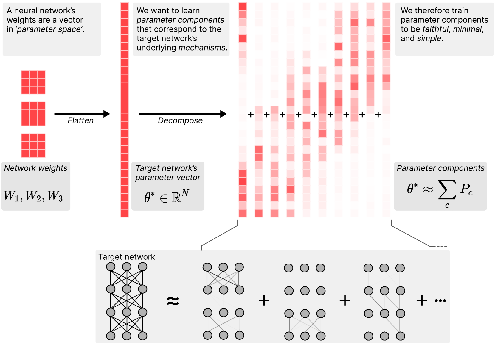
Flatten every weight matrix in a network into one long vector $\theta^* \in \mathbb{R}^N$ . This is the network's position in parameter space, and it is where gradient descent did its work. Braun et al. argue that this is the natural home for mechanisms [3]: the full vector $\theta^*$ does everything the network does, the zero vector does nothing, and vectors in between are candidates for "some but not all of what the network does."

Diagram showing three weight matrices flattened into a single parameter vector, then decomposed into a sum of nine sparser parameter components, with a matching decomposition of the network's connectivity graph below. — Figure 1: A network's weights flattened into a single vector in parameter space, then decomposed into a sum of parameter components. Each component is trained to be faithful, minimal, and simple. From Braun et al., *Interpretability in Parameter Space*. [4]

A vector in parameter space can span whatever it needs to, which is a property activation space lacks. It can cut across neurons, across attention heads, and across layers, because all of those are just coordinates in the same flat vector. A mechanism implemented by three neurons in layer 4 and two heads in layer 7 is a perfectly ordinary parameter vector, whereas an activation-space decomposition has to commit in advance to which layer it lives at.This is also why parameter decomposition is architecture-agnostic in a way that transcoders are not. A transcoder is defined by the sublayer it replaces. A parameter subcomponent does not care which matrix it happens to occupy.

There are infinitely many ways to write $\theta^*$ as a sum, and almost all of them are useless.

What a Good Decomposition Has to Do

Three methods implement this idea, and their names recur throughout this article and the next. Attribution-based Parameter Decomposition (APD) scores components by gradient attribution and keeps the top $k$ on each input, and works on toy models with known ground truth [5]. Stochastic Parameter Decomposition (SPD) drops the attribution step in favour of a learned importance function, and decomposes each matrix into rank-one pieces rather than whole-network vectors [6]. adVersarial Parameter Decomposition (VPD) chooses its ablations adversarially rather than at random, and decomposes a full language model [7].

VPD states the criteria as four properties:

Parameter-faithful: The components sum to the network's parameter vector.
Minimal: As few components as possible are causally important on any given input.
Mechanistically faithful: Every subset of components that contains the causally important ones suffices to compute the network's output on that input.
Simple: Each component uses as little computational machinery as possible.

Parameter faithfulness is what makes this a decomposition rather than an approximation: we are re-coordinatizing the same weights, not fitting a substitute. Minimality is what makes it useful, since a decomposition into one component (the whole network) satisfies everything else trivially. Simplicity rules out the reverse degenerate case.

The other three properties constrain the components one at a time. Mechanistic faithfulness constrains every combination of them at once.

Importance Means Ablatability

How do we decide whether a piece of the network "matters" on an input? The intuitive answer is to score it, by gradient attribution or by patching. Parameter decomposition takes a different route and defines importance directly:

A subcomponent is causally unimportant on an input to the extent that it can be ablated -- scaled down by any amount -- without changing the network's output.

This turns a question about attribution into a question about invariance, and it dodges the well-documented unreliability of gradient attributions [8]. The catch is that checking it exhaustively is hopeless: with $C$ subcomponents there are infinitely many partial-ablation settings, so we cannot verify the property, only sample it.

Ablating "the unimportant components" has two possible readings.

The weak version: the output survives ablating all of them at once. The strong version: the output survives ablating any subset of them, in any combination.

Take two components $\theta_A$ and $\theta_B$ whose contributions cancel. Remove both and nothing changes; remove either one alone and the output breaks. The weak version calls both unimportant, since removing both together is fine. The strong version calls both important, since neither can go on its own.

The strong version is the right one. To call $\theta_A$ and $\theta_B$ unimportant is to claim the model does not need them, and removing either one shows that it does.

Pause and think: why does the weak version fail?

Suppose we allow ourselves the weak version. Here is a decomposition that satisfies it perfectly and teaches us nothing. For every input $x$ in the training set, invent a low-rank component $\theta_x$ , chosen so that running the network with only $\theta_x$ reproduces $f(x \mid \theta^*)$ exactly. Assign it causal importance 1 on $x$ and 0 everywhere else.

Reconstruction is flawless on every training point. But we built these components without ever looking inside the network, and they are a lookup table of the training set. They will not generalize and they describe no mechanism [9].

The strong version kills this. Each $\theta_x$ is marked unimportant on every input except its own, so it demands that the model's output be unchanged when we switch $\theta_x$ partially on during a forward pass for some other input $x'$ . It will not be: $\theta_x$ was fitted to reproduce a completely different output. The lookup table cannot survive being asked to be inert.

Splitting a genuine two-dimensional mechanism into many narrow input-specific subcomponents is the lookup-table move at smaller scale, which is why parameter decomposition should not exhibit feature splitting.

Rank-One Subcomponents

In APD, each parameter component is a vector of the same dimension $N$ as the network's entire parameter vector, carrying one entry per weight across every matrix in the model [10]. That is the picture in Figure 1 taken literally, and it is why the method does not scale: storing $C$ components costs $C$ times the memory of the target network.

SPD decomposes each weight matrix separately into a sum of rank-one matrices, then recovers cross-layer structure afterwards by clustering subcomponents that tend to fire together [11]. For a weight matrix $W \in \mathbb{R}^{d_{\text{in}} \times d_{\text{out}}}$ acting on a row-vector activation $\mathbf{h}$ :

W \approx \sum_{c=1}^{C} \mathbf{v}_c^T \mathbf{u}_c

Each term is the outer product of a read direction $\mathbf{v}_c \in \mathbb{R}^{1 \times d_{\text{in}}}$ and a write direction $\mathbf{u}_c \in \mathbb{R}^{1 \times d_{\text{out}}}$ .The source papers use column vectors and write this as $W_l \approx \sum_c \vec{U}^l_c (\vec{V}^l_c)^\top$ , with $U$ the write direction and $V$ the read direction. Transposed into the row-vector convention this curriculum uses throughout, the read direction is the row vector on the left. The two are the right and left singular vectors of the rank-one matrix respectively. The reason to care about that shape is what happens when activations arrive:

\mathbf{h} \, (\mathbf{v}_c^T \mathbf{u}_c) = (\mathbf{h} \cdot \mathbf{v}_c) \, \mathbf{u}_c

A subcomponent reads one direction out of the incoming activation, collapses it to a scalar, and writes that scalar along one fixed direction. This gives us a natural notion of how strongly a subcomponent engages with an input, its subcomponent activation $a_c = \lVert \mathbf{u}_c \rVert (\mathbf{h} \cdot \mathbf{v}_c)$ , and it makes the later editing story simple, since there is exactly one place to intervene to change what a subcomponent writes.

$C$ can exceed the rank of $W$ . A $768 \times 3072$ matrix can be decomposed into ten thousand rank-one pieces. Without that, the decomposition could not represent computation in superposition, where the network runs more mechanisms than it has dimensions to give them [12].

Parameter faithfulness gets enforced by defining a residual $\Delta$ -component that absorbs whatever the subcomponents miss, and then penalizing it toward zero [13]. The sum is exact by construction; the training pressure is on making the leftover small.

Learning Which Subcomponents Matter

Causal importance is defined by what happens under ablation, so measuring it directly would mean re-running the model under every partial ablation of every combination of subcomponents, at every position of every input. That is the intractability that forced us to sample rather than verify.

SPD proposes predicting the values instead of measuring them. A small network $\Gamma$ reads the target model's hidden activations and outputs $g^l_{b,t,c} \in [0,1]$ for every subcomponent $c$ of every matrix $l$ , at every batch index $b$ and sequence position $t$ [14].

Those predictions become ablation masks $m^l_{b,t,c} \in [g^l_{b,t,c}, 1]$ . Since the predicted importance is itself the lower bound of that interval, it fixes how far the subcomponent may be scaled down. A subcomponent predicted important ( $g = 1$ ) has only one legal mask value, 1, so it is left alone. One predicted unimportant ( $g = 0$ ) can be masked by anything between 0 and 1. We then scale the subcomponents by their masks, assemble new weight matrices, run the model, and require the output to be unchanged:

\mathcal{L}_{\text{masked-recon}} = D\big(f(\mathbf{x} \mid W^1, \ldots, W^L),\; f(\mathbf{x} \mid W'^1(m^1), \ldots, W'^L(m^L))\big)

where $D$ is KL divergence. Nothing yet stops $\Gamma$ from declaring everything important, which would make every mask 1 and this loss zero. An importance-minimality penalty $\sum |g|^p$ supplies the opposing pressure. The equilibrium is a function that marks a subcomponent important only when the model genuinely cannot proceed without it.

Sampling the Masks, and Why Adversarially

Every subcomponent gets its own mask value at every sequence position, and those values are continuous. Even with only a thousand subcomponents, and even collapsing each one to a binary on-or-off choice, checking every setting would take $2^{1000}$ forward passes. So we sample instead, and the choice of sampler decides what the decomposition means.

SPD draws its masks uniformly at random [15]. VPD adds a second sampler that picks masks by gradient ascent on the reconstruction loss, searching for the combination of ablations that pushes the masked model's output furthest from the original model's [16]. The two ask different questions. Random sampling checks whether a typical ablation leaves the output intact; adversarial sampling checks whether the worst one does. Only the second tests the strong version of the requirement -- survive any combination of ablations, not merely a typical one -- which is what rules out the lookup table.

VPD does not fully satisfy the strong version itself. The decomposition holds up under roughly 20 steps of projected gradient descent on the masks (KL divergence 0.83 to the target model) and comes apart under more: 3.84 at 80 steps, 25.3 at 160, 40.2 at 320. There exist ablations of nominally unimportant subcomponents that wreck the model. The authors argue that perfect adversarial robustness is not even the goal, since a sufficiently determined adversary can exploit interference noise in genuinely unused circuitry, but they also say plainly that they would like substantially more robustness than they have. How much is enough is unresolved.

Does It Work?

On toy models with known ground truth, yes. In Elhage et al.'s toy model of superposition, the ground-truth mechanisms are the individual columns of $W$ , each used only when its input feature is active [17]. APD recovers them with mean max cosine similarity $\approx 1$ but shrinks their magnitudes to about 0.9 of the target, an echo of feature shrinkage in SAEs [18]. SPD recovers them with cosine similarity $1.000$ and magnitude ratios of $0.99$ to $1.03$ , and needs far less hyperparameter tuning to get there [19]. SPD also handles two harder variants that defeat APD: a toy model with an identity matrix in the hidden space, and a three-block model of cross-layer distributed representations.

On a real language model there is no ground truth to recover, so the evidence is indirect and rests on how much of the model's behavior the decomposition reproduces. VPD decomposes a four-layer 67M-parameter transformer trained on the Pile, splitting its 24 weight matrices (embeddings excluded) into 38,912 rank-one subcomponents, of which about 10,000 are alive. Each token position uses around 205 of them, or 2.1%. Validation cross-entropy is 2.71 for the target model and 2.72 with the subcomponents unmasked, rising to 2.84 under stochastic masks and 2.94 to 3.02 under various rounded-mask schemes.

Against transcoders, VPD wins on the reconstruction-versus-sparsity tradeoff and scores competitively on intruder detection, an automated interpretability measure that asks an LLM judge to spot the odd example out of a set of activating inputs [20]. It beats per-layer and cross-layer transcoders trained end-to-end, and roughly ties those trained with a layerwise reconstruction loss.

No Feature Splitting

If the strong version is doing its work, extra dictionary capacity should go unused, because there is no way to profit from splitting a mechanism into narrower pieces. That is what happens.

Log-log plot of alive subcomponents against total subcomponent capacity. Per-layer and cross-layer transcoders track the y equals x diagonal, roughly doubling their alive latents when capacity doubles. VPD stays flat near 6,500 across a tenfold range of capacity. — Figure 2: Alive subcomponents against total capacity. Transcoder latent counts scale with dictionary size; VPD's stays flat, leaving the extra capacity unused rather than splitting features into it. From Bushnaq et al., *Interpreting Language Model Parameters*. [21]

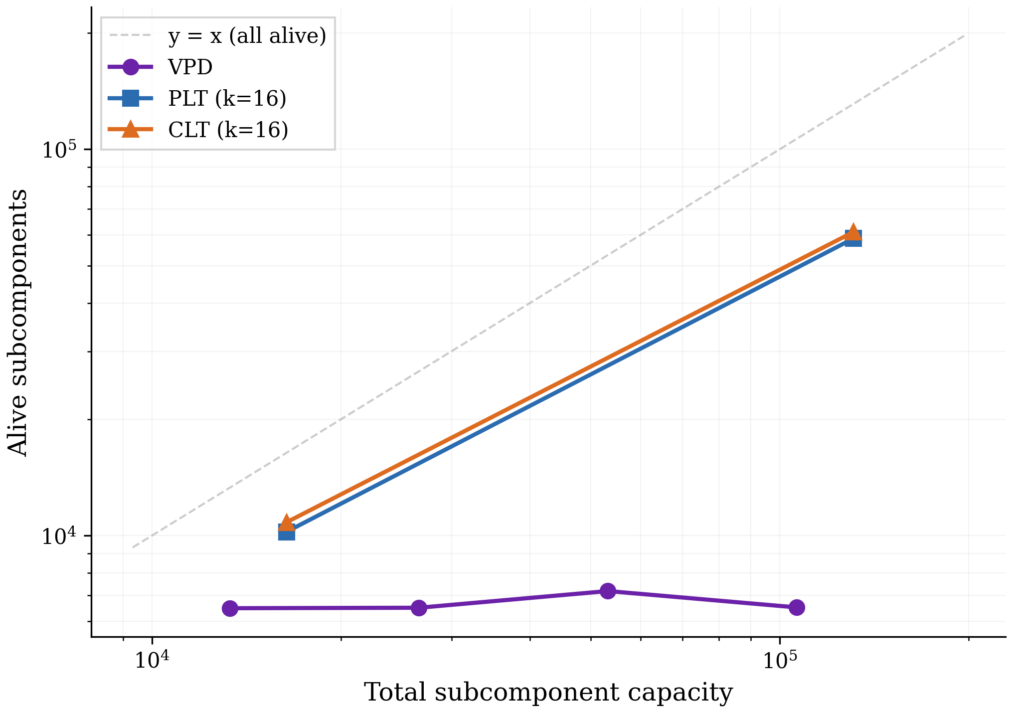
Train VPD at $0.5\times$ , $1\times$ , $2\times$ and $4\times$ the subcomponent capacity and the number of alive subcomponents stays pinned around 6,500 to 7,000, with sparsity and reconstruction essentially unchanged.This sweep counts a subcomponent as alive if it fires at least once every million tokens, which is a stricter test than the mean-causal-importance threshold behind the ~10,000 figure quoted earlier. The two numbers are not directly comparable; what matters here is that this one does not move when capacity does. Per-layer and cross-layer transcoders over the same range scale roughly linearly with dictionary size. The extra capacity is simply left on the floor, which is what it looks like when a method has found a fixed set of mechanisms rather than a resolution knob.

The same qualitative result has held in every model the authors decomposed with SPD or VPD, across toy models with known ground truth and a second small language model trained on SimpleStories.

Pause and think: what would feature splitting look like here?

Suppose VPD did split. With $4\times$ the capacity we would see roughly $4\times$ the alive subcomponents, each firing on a narrower slice of the data, and probably slightly better sparsity and reconstruction as the decomposition specialized. That is exactly the transcoder curve in Figure 2.

Why can it not happen? Take a genuine mechanism spanning a two-dimensional subspace and try to split it into many narrow subcomponents inside that subspace, each aligned with one training activation, with only one marked important at a time. Under causal-importance masking alone this reconstructs beautifully. Under stochastic or adversarial masking, the subcomponents that were not marked important get switched partially on, and their contributions add to the output vector -- making it both too large and pointed the wrong way. The reconstruction collapses. Splitting is only profitable if unmarked subcomponents are guaranteed to stay off, and the sampler removes that guarantee.

What This Does Not Buy Us

Two things are unsettled: the scale at which any of this has been shown to work, and whether the simplicity criterion measures the right thing.

The scale is small. A four-layer 67M-parameter model with roughly 28M non-embedding parameters decomposed, trained on the Pile, is a real language model and not a toy, but it is four orders of magnitude off frontier scale. Nothing here demonstrates that the approach survives the trip.

Rank and firing frequency are proxies for simplicity, not measures of it. Subcomponents are constrained to be rank-one and penalized for firing often, and the authors are explicit that these are guesses at what computational simplicity means. A general-purpose measure of how much machinery a parameter subcomponent uses is an open problem, and it matters because minimizing the description length of the parameters used on a forward pass is not the same thing as minimizing the description length of the forward pass itself.

Looking Ahead

We now have a decomposition of a language model's weights into around ten thousand rank-one pieces, most of which fire on recognizable categories of input. That is a set of units, not an understanding.

The next article puts them to work: attention layers decompose into subcomponents that span multiple heads, which activation-based methods have struggled to do; the QK circuit becomes interactions between pairs of subcomponents; attribution graphs can be built with subcomponents as nodes; and a single rank-one edit is enough to rewrite one small piece of the model's algorithm. That article also carries a methodological result with consequences well beyond parameter decomposition: subnetworks found without an adversary in the loop come out systematically too small.