From Head-Level to Feature-Level Circuits
In the IOI circuit analysis, we traced the mechanism by which GPT-2 Small identifies indirect objects. The circuit had 26 attention heads organized into 7 functional classes. This was a landmark result, but the nodes in that circuit, attention heads, are polysemantic components that participate in many unrelated behaviors. The IOI circuit told us which heads matter, but each head was doing many things beyond the IOI task.
Sparse autoencoders offer a finer-grained candidate unit: a learned direction that is often easier to label than an entire head. Using SAE features as graph nodes can therefore reveal structure hidden by head-level analysis. The tradeoff is that features are not automatically monosemantic, and the SAE's reconstruction error leaves part of the original computation unexplained.
Two lines of work developed this idea. Sparse feature circuits [1]Sparse Feature Circuits: Discovering and Editing Interpretable Causal Graphs in Language Models
Marks, S., Rager, C., Michaud, E. J., et al.
ICLR 2025, 2024 use interventions to test SAE features as circuit nodes. Attribution graphs [2]Circuit Tracing: Revealing Computational Graphs in Language Models
Lindsey, J., Batson, J., Denison, C., et al.
Anthropic, 2025 combine cross-layer transcoders with backward Jacobian tracing to build input-specific feature graphs. Both methods increase resolution, but neither yields a complete map of the original model by default.
Sparse Feature Circuits
Marks et al. (2024) asked whether SAE features could serve as useful nodes in causal circuit graphs. Their sparse feature circuits connect SAE feature discovery with causal intervention, while making the quality of the learned feature basis part of the circuit's assumptions.The term 'sparse feature circuits' emphasizes both properties: activations are sparse, and selected features are connected in a graph. Unlike a head-level graph, this graph depends on a learned decomposition whose features and reconstruction errors must be evaluated.
The pipeline works in four steps:
- Train SAEs on model activations at each layer, producing interpretable features
- Identify causally responsible features using activation patching, for a given behavior, which features matter?
- Build a graph where nodes are SAE features and edges represent causal effects between features across layers
- Prune the graph to retain only edges with significant causal effect
SHIFT: Human-Editable Circuits
An important contribution of Marks et al. is SHIFT (Spurious Human-interpretable Feature Trimming). After discovering a feature circuit, a human inspects the features and identifies those that seem task-irrelevant. Ablating these "spurious" features changes the model's generalization behavior, demonstrating that feature circuits are not just descriptive but editable.
SHIFT bridges the gap between "we found the circuit" and "we can change what the circuit does." This is a concrete step toward using MI for model control, not just model understanding.
Scalable Unsupervised Discovery
Beyond individual circuits, Marks et al. built a scalable unsupervised pipeline that automatically discovers thousands of feature circuits for model behaviors found via SAE feature clustering. No human supervision is needed for the initial discovery phase, human inspection is reserved for validation and editing. This moves circuit discovery from a labor-intensive per-task endeavor toward an automated process.
Limitations of Sparse Feature Circuits
Sparse feature circuits demonstrated the concept, but the approach has important limitations:
- It relies on per-layer SAEs. Features do not naturally cross MLP boundaries, so the circuits cannot trace information through MLP computations.
- Patching is computationally expensive at scale. Each feature must be individually patched, and large models have millions of features.
- Each circuit is task-specific, discovering a new circuit for a new behavior requires running the full pipeline again.
Attribution graphs address these limitations by building a replacement model in which cross-layer transcoders approximate the MLPs, then using Jacobian tracing instead of brute-force patching.
Attribution Graphs
Lindsey et al. (2025) proposed attribution graphs: a method for tracing circuits through language models at the level of individual features [3]Circuit Tracing: Revealing Computational Graphs in Language Models
Lindsey, J., Batson, J., Denison, C., et al.
Anthropic, 2025. The approach has two parts: build a replacement model where MLPs are replaced by cross-layer transcoders, then trace backward from the output through the feature network.
Cross-Layer Transcoders
A regular transcoder reads from one layer's MLP input and writes to that layer's MLP output. A cross-layer transcoder (CLT) extends this idea: it reads from the residual stream at one layer and contributes to all subsequent MLP layers. Features in a CLT can bridge across multiple layers, making cross-layer interactions explicit.Why does bridging matter? Many features persist across layers, for example, 'this token is a proper noun' might be relevant from layer 3 through layer 15. With per-layer SAEs, this feature is rediscovered independently at each layer. With CLTs, it is represented once, and its influence on all downstream layers is captured in a single set of decoder weights.
Cross-Layer Transcoder (CLT): A CLT extends the transcoder concept by reading from the residual stream at one layer and writing to multiple subsequent layers. Features in a CLT can bridge across multiple MLP layers, making cross-layer interactions explicit. When all MLPs in a model are replaced by CLTs, the resulting replacement model has an interpretable sparse structure where feature-to-feature interactions are linear for any given input.
The Replacement Model
The attribution graph method works on a replacement model, not the original:
- Train CLTs to approximate the behavior of all MLP layers simultaneously
- Replace the MLPs with the trained CLTs
- The replacement model behaves similarly to the original but has an interpretable sparse structure
For a specific input, the method treats feature-to-feature effects locally as linear. It holds attention patterns, normalization terms, and active feature gates fixed, then uses a backward Jacobian to compute effects in that local approximation. The derivative can be exact for the replacement model at that point while still failing to capture changes that would alter attention, normalization, or which features activate.
How Graphs Are Constructed
For a specific input:
- Run the replacement model and record all active features, their activations, and the output logits
- Choose a target output, for example, the logit for a specific predicted token. This becomes the root of the graph.
- Trace backward via the Jacobian. For each active feature, compute its linear effect on the target output. Keep features whose effect exceeds a threshold.
- Recurse. For each retained feature, trace backward to find which earlier features (or input embeddings) contributed to its activation. Continue until reaching the input.
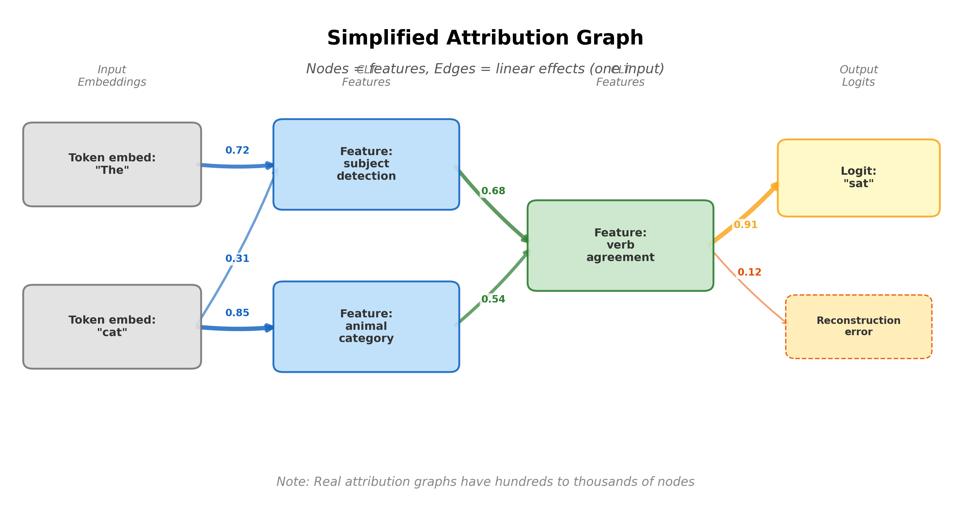
The resulting graph has nodes (CLT features, token embeddings, reconstruction errors, and output logits), edges (linear effects between nodes, weighted by magnitude), and a clear direction from input embeddings through features to output logits.
Recovering Attention Computation
A cross-token edge in an attribution graph says that information at one position influenced a feature at another. In the original construction, the graph held attention patterns fixed. It could show that a "Sally" feature reached the final token, but not which attention heads carried it or why they selected the earlier "Sally" token instead of another position.
Feature-level attention tracing separates those missing questions:
- Which heads carried the edge? Head loadings split an attention-mediated graph edge into contributions from individual heads.
- Why did each head attend there? QK attribution splits a head's attention score into interactions between features at its query and key positions.
The first question concerns the head's OV circuit, which moves information. The second concerns its QK circuit, which selects where to read. Combining them turns an unexplained cross-token edge into a candidate mechanism [4]Tracing Attention Computation Through Feature Interactions
Kamath, H., Ameisen, E., Kauvar, I., et al.
Transformer Circuits Thread, 2025.
Head-Resolved Edges
Suppose source feature is active at position and target feature is active one layer later at position . Let their activations be and , and their residual-stream feature directions be and . Under the local attribution convention used for these graphs, head receives the loading
where is the observed attention weight from the target position to the source position. Summing across heads gives the attention-mediated part of the edge. The scalar measures how well the information written by head from the source direction aligns with the target direction.
Edges between cross-layer transcoder features can span several layers, collapsing exponentially many possible sequences of heads into one weight. To make head loadings tractable, the method checkpoints the residual stream with sparse autoencoder (SAE) features after each layer. Each adjacent-layer edge can then contain several heads, but it cannot hide a multi-layer chain of heads. This gains head-level resolution while giving up the clean replacement-model interpretation of CLT encoder weights.Residual-stream SAE encoders infer which features are active; they are not themselves weights in a replacement computation. Head loadings should therefore be treated as local attributions and checked with interventions, not as a complete causal factorization.
Head loading: The portion of a feature-to-feature edge attributed to one attention head's observed attention weight and OV transformation.
Feature-Pair QK Attribution
A head loading identifies a carrier, but an attention weight alone does not explain why the head chose that source. The pre-softmax score is bilinear in the residual streams at query position and key position :
Residual-stream SAEs express each activation as active feature directions plus a bias and reconstruction error:
Substituting these sums into the bilinear score produces one term for every query-feature and key-feature pair:
The full score also contains feature-bias, feature-error, bias-error, and error-error interactions. Retaining those terms makes the decomposition add back to the score represented by the SAE reconstruction. Large positive terms favor attending from to ; negative terms suppress that pairing.
QK attribution: A feature-pair decomposition of an attention head's pre-softmax score at one query-key position pair.
QK attribution is distinct from the AtP* QK fix. AtP* recomputes how attention changes under a patch so that a saturated softmax does not hide important nodes. QK attribution holds one observed prompt in view and explains which feature pairs contributed to its score.
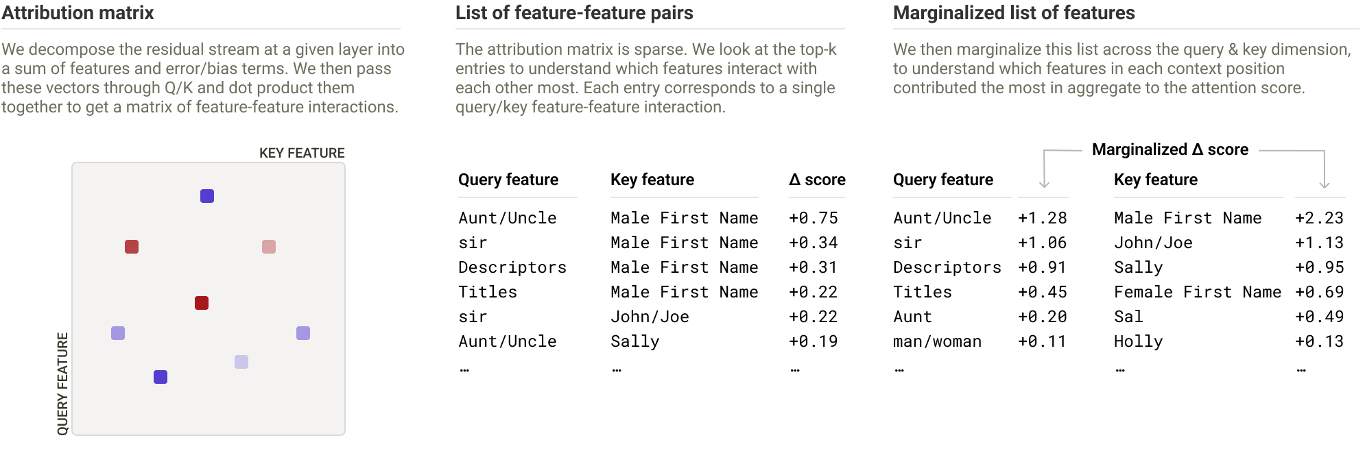
Kamath, H., Ameisen, E., Kauvar, I., et al.
Transformer Circuits Thread, 2025
QK attribution explains a score, while the softmax attention pattern compares that score with every competing key position. Understanding why a head attended to one token can therefore require inspecting positive terms at the selected key and negative terms at alternatives. The method exposes those terms but does not automatically decide which counterfactual positions matter.
Worked Example: The Features Behind Induction
Consider the prompt "I always loved visiting Aunt Sally. Whenever I was feeling sad, Aunt", which Claude 3.5 Haiku completes with "Sally." A feature graph can reveal an OV route that copies information from the earlier "Sally" token. That still leaves the selection mechanism unexplained: why did the relevant heads attend to "Sally"?
Head loadings first identify the small set of heads mediating the cross-token edges. Their QK attributions show query-side features for "Aunt" or family roles interacting with two kinds of key-side features:
- Features representing names in general or "Sally" specifically
- Features representing that a token is the name following "Aunt" or "Uncle"
The two interactions reveal parallel heuristics. One searches broadly for a name; the other searches for a name bound to the relevant family role. An earlier previous-token head helps construct the role-linked feature on "Sally," connecting the familiar induction circuit to feature-level QK geometry.
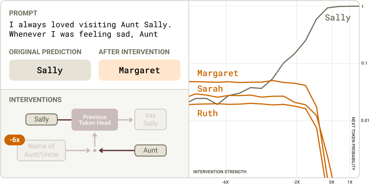
Kamath, H., Ameisen, E., Kauvar, I., et al.
Transformer Circuits Thread, 2025
The intervention changes only the selected feature contribution inside the relevant QK circuits. Its effect on both attention and the next-token prediction is stronger evidence than reading feature labels from the attribution matrix alone. It remains evidence about one prompt family and model, not proof that every induction head implements the same feature interactions.
What Attribution Graphs Can Reveal
Attribution graphs have been applied to Claude 3.5 Haiku across multi-step reasoning, multilingual processing, and constrained generation [7]On the Biology of a Large Language Model
Anthropic
Anthropic, 2025. These examples illustrate recurring analytical capabilities rather than defining separate methods.
Multi-Step Reasoning
When asked "What is the capital of the country containing the city of Dallas?", the attribution graph reveals a chain of features:
- A "Dallas" feature activates, recognizing the city
- This activates a "Texas" feature, a geographic association
- The "Texas" feature activates a "United States" feature, state-to-country mapping
- The "United States" feature activates a "Washington D.C." feature, capital knowledge
Each step appears as a distinct feature-to-feature connection in the replacement model's attribution graph. For this prompt, the graph supports a multi-step route through intermediate geographic features rather than one attributed edge from “Dallas” to “Washington D.C.” Because the graph is sparse, input-specific, and built from an approximation, it is evidence for that route rather than an exhaustive transcript of the original model.
Multilingual Processing
In one multilingual case study, early graph features were associated with language-specific tokens and grammar, while some intermediate features responded across languages to related meanings. Later features were again tied to the output language. This pattern is consistent with a partly shared semantic representation, but “language-agnostic” should not be read as proof that the features discard every language-specific cue.
Poetry and Rhyme
When completing a poem where the next word must rhyme, the attribution graph reveals two parallel pathways: a semantic pathway encoding the meaning and theme of the poem, and a phonetic pathway encoding the sound pattern and rhyme constraint. These pathways converge at the output, producing a word that satisfies both meaning and rhyme, a concrete example of how multiple computational goals are solved in parallel through the feature network.
Pause and think: Per-input vs. global circuits
Attribution graphs show a chain of features for multi-step reasoning: Dallas, Texas, United States, Washington D.C. But this is the graph for one specific input. Would the model use the same chain for "What is the capital of the country containing Houston?" Would the intermediate features be identical?
What would it take to go from per-input graphs to a general understanding of how the model does geographic reasoning? You would need to run attribution graphs on many similar prompts, align the resulting graphs, and look for shared structure. This aggregation problem, going from many individual circuit traces to a universal circuit description, is not yet solved and remains one of the field's key open challenges.
Limitations of Current Circuit Tracing
Per-Input, Not Global
One central limitation is that attribution graphs are per-input. Each graph describes one prompt, and prompts expressing the same behavior can produce different graphs. There is no guarantee that the graph for "Dallas" generalizes to "Houston." A broader account requires comparing traces across many inputs and testing which structure persists.A single trace is closer to a case study than a general theory. Repeated traces can reveal recurring structure, but the aggregation procedure and the relevant input distribution both affect the conclusion.
CLT Approximation Quality
The replacement model is an approximation. CLTs are trained to match MLP behavior, but the match is imperfect. Reconstruction error nodes in the graph capture what the CLTs miss. If the CLTs systematically fail to capture certain computations, those computations will be invisible in the graph. The quality of the attribution graph is bounded by the quality of the CLT approximation.
Active Features Only
Attribution graphs show only active features, those that fire on the given input. Features that are inhibited (actively suppressed) may not appear. Features that would be relevant but happen to be inactive on this input are invisible. The graph shows what the model does, not what it could have done. Contrast this with the IOI analysis, where Backup Name Mover heads were discovered through ablation of the primary pathway.
Attention Scores, Softmax, and Normalization
Head loadings and QK attribution repair two omissions in the original graphs: they identify which heads mediate an edge and which query-key feature interactions contribute to an observed pre-softmax score. They do not turn the full graph into an exact nonlinear account.
The backward attribution graph still conditions on the current input and locally fixed attention patterns. The QK decomposition explains each score before softmax, while the attention pattern depends on competition among scores at all key positions. Layer normalization also changes the vectors entering QK computation and must be handled through a local linearization. An intervention can therefore change the attention pattern, normalization denominator, or active feature set in ways that the original graph edges do not predict.
Computing every query-key feature interaction also scales quadratically with context length before accounting for the number of active feature pairs. Long-context use will require pruning to important graph edges, heads, and token pairs.
The Evolution of Circuit Analysis
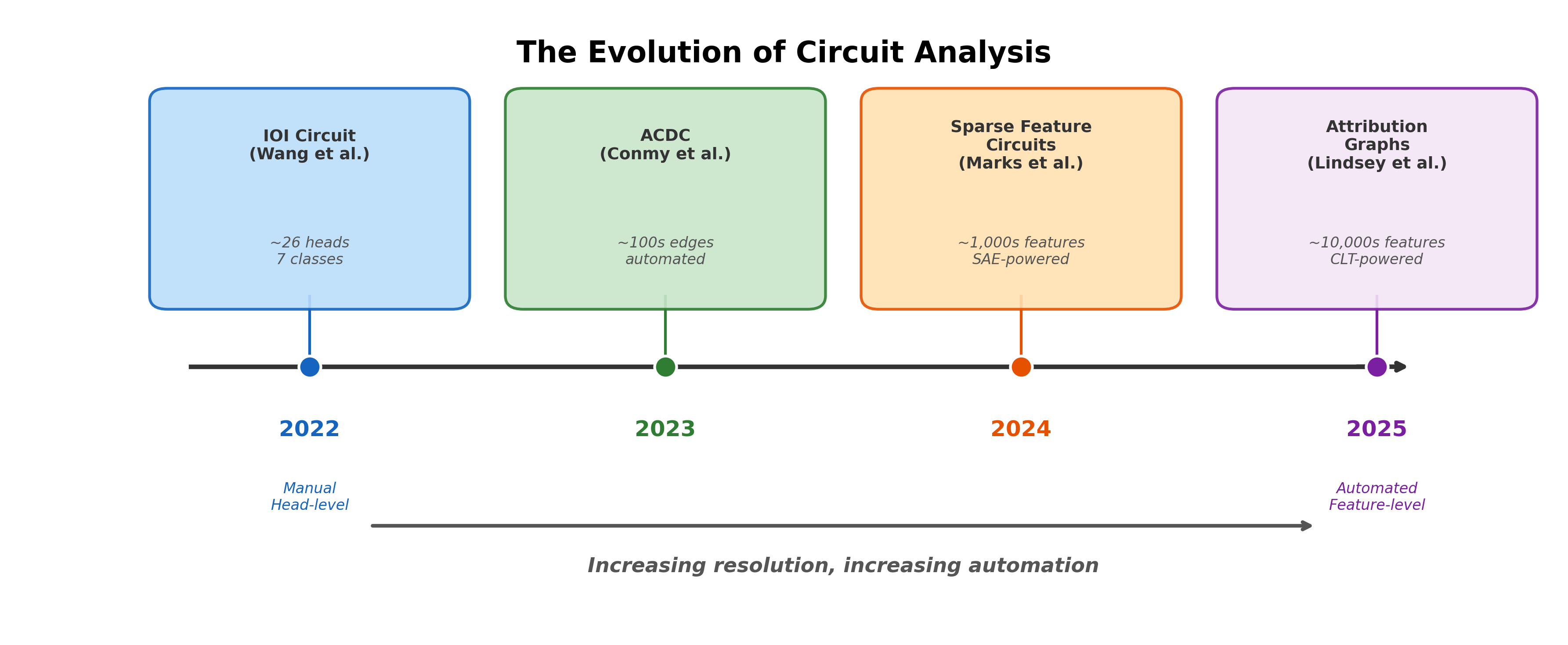
- 2022: Manual head-level analysis (IOI). 26 heads, 7 classes. Months of researcher effort for one circuit in a 117M-parameter model. Nodes are polysemantic attention heads.
- 2023: Automated head-level analysis (ACDC). Conmy et al. automated path patching [8]Towards Automated Circuit Discovery for Mechanistic Interpretability
Conmy, A., Mavor-Parker, A. N., Lynch, A., et al.
NeurIPS, 2023. Still head-level granularity, but the search is algorithmic rather than manual. - 2024: Feature-level circuits (Marks et al.). SAE features as circuit nodes [9]Sparse Feature Circuits: Discovering and Editing Interpretable Causal Graphs in Language Models
Marks, S., Rager, C., Michaud, E. J., et al.
ICLR 2025, 2024. Higher resolution than heads, but still per-layer and patching-based. - 2025: Attribution graphs (Lindsey et al.). Cross-layer transcoders, Jacobian tracing, thousands of features [10]Circuit Tracing: Revealing Computational Graphs in Language Models
Lindsey, J., Batson, J., Denison, C., et al.
Anthropic, 2025. The highest resolution yet, applied to production-scale models. - 2025: Attention-resolved graphs. Head loadings expose which heads carry feature edges, while QK attribution explains their pre-softmax scores through query-key feature interactions [11]Tracing Attention Computation Through Feature Interactions
Kamath, H., Ameisen, E., Kauvar, I., et al.
Transformer Circuits Thread, 2025.
Each step gained something and lost something. Higher resolution brings more detail but also more complexity. Automation brings scale but also requires more careful validation. And the fundamental challenge, going from per-input analysis to global circuit understanding, remains across all generations.Both IOI patching and attribution graphs are evaluated on selected inputs and behaviors. The reported IOI circuit did not recover all measured performance, and attribution graphs inherit reconstruction error from their replacement model. A circuit diagram is therefore evidence about a computation, not a certificate that the computation is fully understood.
Pause and think: What would global circuits look like?
Attribution graphs give us a per-input circuit. Imagine we could somehow aggregate thousands of attribution graphs for the same behavior into a single "global" circuit. What would that circuit look like? Would it have the same structure as individual attribution graphs, or would it be fundamentally different?
Consider that different inputs might activate different subsets of features, use different intermediate representations, or follow different computational paths to the same output. A global circuit might need to represent branching, optional paths, and input-dependent routing, structures that are absent from individual attribution graphs. This is an open research question.
From One Model to Many
Attribution graphs have moved circuit analysis from tens of polysemantic heads to thousands of sparse features, while attention-resolved tracing recovers some of the routing that frozen-attention replacements hide. The additional resolution does not remove the need for causal validation: every graph is conditional on an input, a replacement model, an attribution rule, and a pruning threshold.
The next question is whether a circuit learned in one model tells us anything about another. Universality Across Models examines the evidence that independently trained networks converge on analogous features and mechanisms, and the stronger claim that their internal representations can be put into one-to-one correspondence.