Additive Writes Become Logit Contributions
Every component in a transformer writes additively into the residual stream. The final residual stream is a sum of contributions: the token embedding, each attention head's output, and each MLP layer's output. Because the unembedding matrix maps this final residual stream to output logits through a linear operation, the logits are also a sum of contributions. Each component's effect on the output can be measured independently.
This observation is the foundation of direct logit attribution (DLA), introduced in the mathematical framework for transformer circuits [1]A Mathematical Framework for Transformer Circuits
Elhage, N., Nanda, N., Olsson, C., et al.
Anthropic, 2021. Projecting each component's write onto an unembedding or logit-difference direction measures its direct contribution in one forward pass. It is a screening tool for causal hypotheses, not a complete allocation of responsibility.
Direct Logit Attribution (DLA): Direct logit attribution decomposes the model's output logits as a sum of per-component contributions. For attention head predicting token , the attribution is: , where is the head's output written to the residual stream. A positive value means the head promotes token ; a negative value means it suppresses .
The Decomposition
To see how DLA works, consider the structure of the final residual stream. After all layers have processed, the residual stream at a given position is:
where is the output of attention head at layer , and is the output of MLP layer . The output logits are computed by multiplying this sum by the unembedding matrix:
Because matrix multiplication distributes over addition, the logits decompose into a sum of per-component terms:
Each term in this sum is one component's direct contribution before final normalization. In a model with a final LayerNorm, raw projections do not sum directly to the logits. A common implementation uses the normalization scale from the full forward pass and applies that same fixed affine map to every component. Those adjusted terms can sum to the observed logits, apart from separately handled biases, but they do not describe how the normalization scale would change under an intervention.
For a specific prediction, we often care about the logit difference between two competing tokens. In the Indirect Object Identification (IOI) task studied by Wang et al. [2]Interpretability in the Wild: a Circuit for Indirect Object Identification in GPT-2 Small
Wang, K., Variengien, A., Conmy, A., et al.
arXiv, 2022, the model must choose between two names (say, Mary and John). The relevant quantity is:
Each component's contribution to this logit difference is:
The vector defines a single direction in residual stream space. Projecting each component's output onto this direction tells us whether that component pushes toward predicting Mary (positive) or John (negative), and by how much.
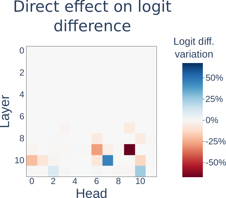
Wang, K., Variengien, A., Conmy, A., et al.
arXiv, 2022
Per-Token Attribution: A Screening Tool
Direct logit attribution (DLA) is often the first screening step in circuit discovery:
- Run the model on a prompt where you know the correct next token.
- Cache every component's output at the position of interest.
- Compute each component's DLA for the correct token (or the logit difference between correct and incorrect).
- Sort components by DLA magnitude to find the biggest contributors.
In the indirect object identification (IOI) analysis, the Name Mover heads (9.9, 10.0, 9.6) had the largest positive DLA for the correct name, narrowing 144 candidate heads to a small set for further study [4]Interpretability in the Wild: a Circuit for Indirect Object Identification in GPT-2 Small
Wang, K., Variengien, A., Conmy, A., et al.
arXiv, 2022. Testing every head individually with causal methods would have required many more model runs.DLA also helped identify induction heads in the mathematical framework analysis. For sequences of the form [A][B]...[A], one head had an unusually large positive direct contribution to the repeated continuation, motivating study of its two-step mechanism.
DLA is useful for screening because it needs one forward pass followed by dot products, with no additional model runs or gradients. It quickly ranks components by direct contribution. “Direct” matters: a small value can hide a large indirect effect, and a large value need not survive downstream processing.
Pause and think: Interpreting DLA values
Suppose you run DLA on a prompt and find that head 7.3 has a DLA of +2.1 for the correct token, while head 10.7 has a DLA of -1.8. What does each value mean? If you summed the DLA values of all components, what would you get?
Head 7.3 has a positive direct contribution of 2.1 to the chosen token's logit, while head 10.7 contributes -1.8. Before final normalization, summing every component recovers the corresponding raw-logit contribution. With LayerNorm, the equality requires a consistent decomposition that uses the full run's normalization factors and accounts for biases.
Reading Attention Patterns
DLA tells us how much each head contributes to the prediction, but not how it computes that contribution. To understand the mechanism, we need to look at what each important head is actually doing. One natural tool is visualizing the head's attention pattern.
An attention pattern is an matrix where entry gives how much position attends to position . Each row sums to 1, forming a probability distribution over source positions. Visualized as a heatmap, these patterns reveal what a head is "looking at."
Previous-token, induction, anchor-token, and approximately uniform patterns recur across models:
Diagonal pattern. Each position attends primarily to the token immediately before it. This produces a shifted diagonal line in the attention matrix. Heads with this pattern are called previous token heads, and they play the first role in induction circuits by writing "my predecessor was token X" into the residual stream.
Off-diagonal stripe. The head attends to specific tokens based on content matching, producing attention that jumps across positions. Induction heads display this pattern: at the second occurrence of a token, they attend not to the repeated token itself, but to the token that followed the previous occurrence.
Column pattern. Many destination positions attend to the same source token, creating a vertical stripe. Common targets include the beginning-of-sequence token, punctuation, or other structural markers.A beginning-of-sequence column can have several meanings. The head might read a useful value from that position, use it as an attention sink when no content match is needed, or contribute an approximately constant write. The OV circuit and interventions distinguish these possibilities.
Uniform pattern. Attention is distributed roughly equally over the positions available under the causal mask. This is consistent with averaging values, but the result depends on what the OV circuit extracts and writes.
Each pattern type provides a clue about the head's function. Diagonal patterns suggest local or positional processing. Off-diagonal stripes suggest content-based lookup. Column patterns suggest anchor token computation. Uniform patterns suggest global averaging.
Pause and think: What attention patterns cannot tell you
You are analyzing a model processing "Alice gave the book to Bob." Head A attends from "to" strongly to "Alice." Head B also attends from "to" strongly to "Alice," with an identical attention pattern. Can you conclude that both heads are doing the same thing?
No. Attention patterns come from the QK circuit and show where a head looks. The what, what information the head moves, comes from the OV circuit. Two heads with identical attention patterns but different OV matrices can have completely different effects on the output. Head A might copy Alice's identity to the residual stream while Head B might suppress Alice's identity. To understand a head's role, you need both the attention pattern and the OV circuit analysis.
The Limitation: Observation, Not Causation
DLA is a powerful screening tool, but it has a fundamental limitation. It measures a component's direct projection onto an output direction. The additive decomposition is exact before final normalization, but it does not include indirect effects mediated by later components or allocate interactions among components.
Later components can counteract earlier writes. Suppose head 5.3 writes a strong positive signal for “Paris,” but a later MLP writes in the opposite direction. DLA records both direct writes; it does not tell us how the earlier write changed the later MLP's computation.The distinction is between a direct residual-stream contribution and a total causal effect. Later layers can amplify, redirect, or cancel earlier information, and they may themselves behave differently when an earlier component is changed.
A large direct contribution does not show that the model relies on that component. Downstream layers may erase the information, or another component may supply a redundant path. DLA therefore supports an observational claim about what was written, not a causal claim about what the computation required.
To test a causal hypothesis, use an intervention such as activation patching. If replacing a component changes the chosen metric, that component mediates some effect under the specific patch. A small effect can instead reflect redundancy, self-repair, an unsuitable corruption, or a component that simply is not important in that context.
DLA and attention-pattern analysis are observational tools. They show what components write directly and where attention is routed. Moving from “this component writes a signal” to a causal claim requires a well-designed intervention, a clear metric, and attention to redundancy and distribution shift.