The L1 Problem
The sparse autoencoders that produced the scaling monosemanticity results use an L1 penalty on feature activations to encourage sparsity. The training objective is:
The L1 term pushes feature activations toward zero, encouraging sparse representations. This is the standard approach, and it works well enough to produce millions of interpretable features. But it has a fundamental problem.
The L1 penalty does not just encourage sparsity. It also distorts feature magnitudes. The model can reduce by making all activations smaller, even when they should be large. This creates shrinkage: systematic underestimation of how active each feature truly is. The sparsity penalty trades reconstruction accuracy for a lower sparsity cost, and the features we recover are biased as a result.Shrinkage from L1 regularization is a well-known phenomenon in statistics, where it appears in the context of LASSO regression. The LASSO estimator produces biased coefficient estimates that are systematically too small. SAEs inherit this same bias because they use the same L1 penalty for sparsity.
The core issue is that L1 conflates two distinct questions:
- Which features are active? This is the selection decision, a binary on/off question.
- How active are they? This is the magnitude estimation, a continuous value.
L1 penalizes both simultaneously. A feature that should be active with magnitude 5.0 might only reach 3.0 because the L1 penalty pushes it down. The selection might be correct (the feature is active), but the magnitude is wrong (it is too small). This distortion flows into the reconstructed activation and degrades the SAE's fidelity.
What we actually want is L0 sparsity: a count of how many features are active.
counts active features without penalizing their magnitudes. Because this count changes discontinuously at zero, ordinary gradient descent cannot optimize it directly. The norm supplies a differentiable convex surrogate, at the cost of shrinking nonzero magnitudes.
The history of SAE variants is the story of getting closer to direct L0 optimization. Each variant addresses a specific shortcoming of its predecessor, and the overall trajectory moves from "L1 as a rough proxy" to "something much closer to what we actually want."
Gated SAEs: Separate Selection from Magnitude
Gated SAE: An SAE architecture that uses two separate pathways, a gating pathway for feature selection and a magnitude pathway for activation estimation, so that the L1 sparsity penalty applies only to the selection decision and cannot distort magnitude estimates [1]Improving Dictionary Learning with Gated Sparse Autoencoders
Rajamanoharan, S., Conmy, A., Smith, L., et al.
NeurIPS, 2024.
Rajamanoharan et al. (2024) identified the core problem: vanilla SAEs use a single pathway for both selection and magnitude, which means the L1 penalty distorts both [2]Improving Dictionary Learning with Gated Sparse Autoencoders
Rajamanoharan, S., Conmy, A., Smith, L., et al.
NeurIPS, 2024. Their solution is to decouple them into two separate pathways.
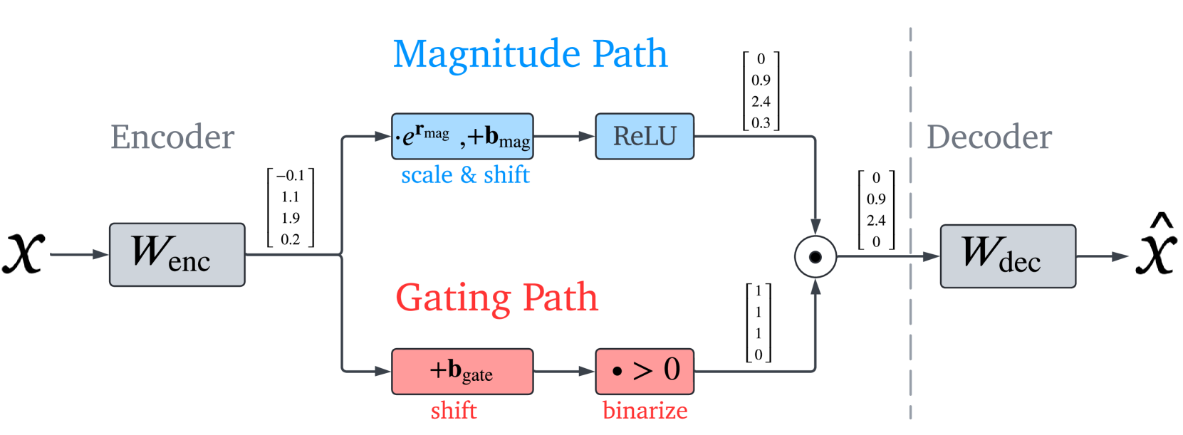
Rajamanoharan, S., Conmy, A., Smith, L., et al.
NeurIPS, 2024
The gating pathway makes the binary on/off decision for each feature. A learned linear transformation followed by a threshold determines which features are active. The L1 penalty applies only here, encouraging the gate to be sparse.
The magnitude pathway estimates how active each feature is, using a separate linear transformation. Because this pathway is free from the L1 penalty, it can estimate magnitudes without bias.
The combined activation is:
where is elementwise multiplication and is the indicator function. The gate decides which features are on. The magnitude pathway decides how strong they are. The sparsity penalty cannot distort magnitudes because it only touches the gate.
In the reported comparison, Gated SAEs improve the reconstruction–sparsity frontier over the vanilla baseline: at matched (number of active features), they achieve lower reconstruction error. This is a result for the tested training setup, not a guarantee over every dataset and architecture.
TopK SAEs: Direct Sparsity Enforcement
TopK SAE: An SAE architecture that enforces exact sparsity by keeping only the largest pre-activations and zeroing out the rest, eliminating the need for an L1 penalty entirely [4]Scaling and Evaluating Sparse Autoencoders
Gao, L., Dupre la Tour, T., Tillman, H., et al.
ICLR 2025, 2024.
Gao et al. (2024) took a more direct approach: skip L1 entirely [5]Scaling and Evaluating Sparse Autoencoders
Gao, L., Dupre la Tour, T., Tillman, H., et al.
ICLR 2025, 2024. The TopK activation function retains only the largest pre-activations and sets all others to zero:
where is the pre-activation for feature .
Sparsity is exactly by construction. There is no L1 penalty at all, so there is no shrinkage. The features that survive the selection pass through with their full magnitudes intact. The loss function is simply reconstruction error, no sparsity term needed.
Gao et al. trained TopK SAEs with as many as 16 million latents on GPT-4 activations. Their measured reconstruction and sparsity metrics followed regular scaling trends as dictionary size and compute increased.Large SAE studies from OpenAI and Anthropic both report smoother improvement on some proxy metrics as dictionary size grows. Whether semantic quality follows the same trend depends on the evaluation; lower reconstruction loss does not by itself make a feature easier to interpret.
The limitation of TopK is rigidity: every token uses exactly features, regardless of whether that token is simple or complex. A common function word like "the" might need only 5 features, while a technical term in a specialized context might need 50. TopK forces both to use the same number, which is likely suboptimal.
Pause and think: Fixed vs. adaptive sparsity
TopK SAEs enforce the same number of active features for every input. Is this reasonable? Think about a language model processing the sentence "The cat sat on the mat." Would you expect every token to require the same number of features? What about a sentence like "The intricate geopolitical ramifications of the treaty were debated at the symposium"? How might you design an SAE that adapts its sparsity to the input?
JumpReLU SAEs: Learnable Thresholds
JumpReLU SAE: An SAE architecture with a discontinuous activation function that uses a learnable threshold per feature, zeroing pre-activations below the threshold and passing those above through unchanged, enabling direct L0 optimization via straight-through estimators [6]Jumping Ahead: Improving Reconstruction Fidelity with JumpReLU Sparse Autoencoders
Rajamanoharan, S., Lieberum, T., Sonnerat, N., et al.
arXiv, 2024.
Rajamanoharan et al. (2024) introduced a different solution: a discontinuous activation function with a learnable threshold [7]Jumping Ahead: Improving Reconstruction Fidelity with JumpReLU Sparse Autoencoders
Rajamanoharan, S., Lieberum, T., Sonnerat, N., et al.
arXiv, 2024:
Each feature has its own threshold . Pre-activations below the threshold are zeroed; those above pass through unchanged. There is no shrinkage because the surviving activations are not modified at all. And unlike TopK, different inputs can have different numbers of active features, because the threshold is per-feature rather than global.
The challenge is training. The JumpReLU function is discontinuous at , which blocks gradient flow. Rajamanoharan et al. use straight-through estimators (STEs) to handle this: they replace the discontinuous gradient with a smooth approximation during the backward pass, while keeping the discontinuous function during the forward pass. This allows the thresholds to be learned end-to-end.
The loss function directly optimizes L0 sparsity:
No L1 term at all. No shrinkage. No magnitude distortion. The L0 penalty counts active features, and the STE provides the gradients needed to train the thresholds that control which features are active.
On Gemma 2 9B, JumpReLU achieved better reconstruction fidelity at a given sparsity level than the tested Gated and TopK sparse autoencoders.
The Evolution at a Glance
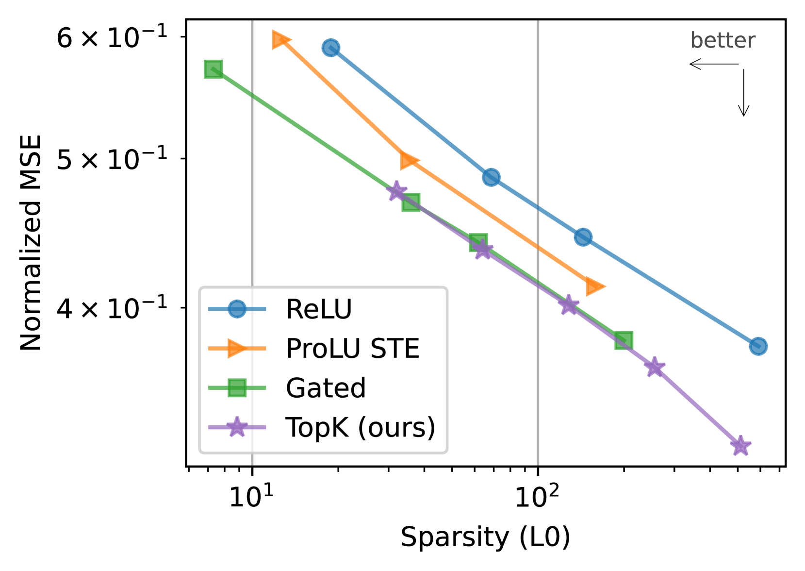
Gao, L., Dupre la Tour, T., Tillman, H., et al.
ICLR 2025, 2024
The four SAE architectures form an iterative improvement story:
Vanilla L1: Simple but biased. The L1 penalty introduces shrinkage that distorts feature magnitudes.
Gated: Separate selection from magnitude. The sparsity penalty applies only to the gate, leaving magnitudes unbiased. A Pareto improvement over vanilla.
TopK: Enforce exact sparsity directly. No L1 penalty at all. But fixed for every input may be suboptimal.
JumpReLU: Learnable per-feature thresholds with direct L0 optimization. Adaptive sparsity, no shrinkage, state-of-the-art performance.
These variants move from L1 as a proxy for sparsity toward more direct control of the active set. Each targets a known optimization problem in an earlier objective. Better reconstruction and sparsity metrics are useful, but they leave the central evaluation question open: do the learned latents support better interpretability work?
Training Objectives: MSE vs. End-to-End
All the architectural variants above share a common training setup: they optimize mean squared error (MSE) on precomputed, shuffled activations. The SAE learns to reconstruct activations as faithfully as possible, and we hope that faithful reconstruction translates to faithful model behavior. But the metric we actually care about is different: the increase in cross-entropy loss when SAE reconstructions replace the original activations during inference.
This creates a mismatch. MSE weights activation-space errors by their squared magnitude, while different directions can have very different effects on the model's predictions. Braun et al. (2024) proposed end-to-end (E2E) SAE training to reduce that mismatch: use a combined KL-divergence and MSE loss so the SAE receives feedback from the model's output distribution [9]Identifying Functionally Important Features with End-to-End Sparse Dictionary Learning
Braun, D., Taylor, J., Goldowsky-Dill, N., Sharkey, L.
arXiv, 2024. The KL term emphasizes reconstruction errors that change predictions, while the MSE term stabilizes reconstruction. In the reported experiments, E2E training improved the sparsity-fidelity tradeoff but required language-model forward passes during every training step. It also prevented activation shuffling and reduced opportunities to amortize training across layers, making it substantially more expensive than training on cached activations.
Karvonen (2025) found that much of the end-to-end (E2E) benefit could be recovered in the tested setup by training normally with mean squared error (MSE), then applying a brief Kullback–Leibler-plus-MSE fine-tuning step for 25 million tokens, about 0.5% to 10% of the comparison training budgets [10]Revisiting End-To-End Sparse Autoencoder Training: A Short Finetune Is All You Need
Karvonen, A.
arXiv, 2025. The procedure reduced the measured cross-entropy loss gap by 20% to 50%. Several lightweight alternatives, including low-rank adaptation (LoRA) on the language model and linear adapters after the SAE encoder, recovered a similar fraction individually, while their benefits did not stack. This non-additivity is consistent with a shared, correctable error pattern, although it does not uniquely identify one.
A short fine-tuning step can therefore improve behavioral fidelity at lower cost than fully end-to-end training in this setup. That can reduce reconstruction-error nodes in circuit analysis, but it does not reveal a uniquely true circuit. The accompanying SAEBench results reinforce the broader evaluation lesson: lower cross-entropy loss does not consistently produce better supervised interpretability metrics. Benefits depend on the SAE architecture and the downstream task.
Evaluating SAEs: SAEBench
Most SAE work evaluates progress using unsupervised proxy metrics: reconstruction loss (), L0 sparsity (how many features are active), and explained variance (what fraction of activation variance the SAE captures). These are easy to compute and clearly defined. But do they measure what we actually care about?
Karvonen et al. (2025) built SAEBench, an evaluation suite organized around a more direct question: can SAE features help with specific interpretability tasks [11]SAEBench: A Comprehensive Benchmark for Sparse Autoencoders in Language Model Interpretability
Karvonen, A., Rager, C., Lin, J., et al.
arXiv, 2025?
SAEBench includes eight metrics spanning four categories:
- Concept detection: Can SAE features identify known concepts like gender, profession, and sentiment?
- Interpretability: Are features human-interpretable? Do automated descriptions match activation patterns?
- Feature disentanglement: Do individual features correspond to individual concepts, or are related concepts entangled across multiple features?
- Reconstruction quality: The standard proxy metrics, included for comparison.
RAVEL supplies a causal test of feature disentanglement [12]RAVEL: Evaluating Interpretability Methods on Disentangling Language Model Representations
Huang, J., Wu, Z., Potts, C., Geva, M., Geiger, A.
ACL, 2024. A proposed feature receives a Cause score for changing its target attribute under an interchange intervention and an Isolate score for preserving neighboring attributes. On the original Llama2-7B benchmark, the tested vanilla SAE reached 48.6% and 46.8% combined disentanglement on the entity and context splits, compared with 60.1% and 65.6% for Multi-task Distributed Alignment Search. Principal Component Analysis scored lower still. This is a scoped comparison between particular featurizers and feature-selection procedures, not a general ranking of every SAE against every supervised method.
Across these benchmarks, proxy metrics did not reliably predict task performance. SAE variants with better reconstruction loss or L0 sparsity did not consistently improve concept detection, description quality, or disentanglement. A JumpReLU SAE with better reconstruction than a vanilla SAE, for example, need not be better at detecting a labeled concept such as deception.SAEBench often found Gated, TopK, and JumpReLU SAEs difficult to distinguish on the evaluated practical metrics even when their proxy metrics differed. Reconstruction and sparsity describe important properties of an SAE, but they are insufficient to establish usefulness for a particular interpretability task.
This result does not invalidate the architectural improvements. Better reconstruction and lower shrinkage address real failure modes. It does show that reconstruction loss alone is insufficient for many downstream tasks, so an SAE should also be evaluated on the use for which it was chosen.
The field lacks consensus on what "a good SAE" means in practice. Proxy metrics are insufficient. Task-specific evaluation is necessary but depends on having ground-truth concepts to test against. Building better evaluation methods remains one of the most important open problems in SAE research.
Limitations That Affect Interpretation
SAEs have produced features with useful labels and causal effects, alongside steadily improving architectures. The same outputs can still mislead when features split, absorb one another, remain dead, or support incomplete labels. Any analysis built on an SAE inherits these failure modes.
Feature Absorption
Chanin et al. (2024) identified feature absorption: a failure mode where hierarchical features collapse [13]A is for Absorption: Studying Feature Splitting and Absorption in Sparse Autoencoders
Chanin, D., Wilken-Smith, J., Dulka, T., et al.
NeurIPS Workshop, 2024.
Consider a hierarchy of features:
- Parent feature: "word starts with the letter A"
- Child feature: "the word Apple"
In a well-behaved SAE, both features should fire for "Apple", the parent (starts with A) and the child (the specific word). But absorption causes the parent feature to not fire for inputs that match a child feature.
Why does this happen? The sparsity objective incentivizes the SAE to reduce the number of active features per input. If "Apple" can be explained by the "Apple" feature alone, the SAE learns to suppress the "starts with A" feature for that input. This reduces L0 by one. The result: the parent feature "starts with A" fires for "Axolotl" and "Azure" but not for "Apple", even though "Apple" starts with A. The parent feature has been absorbed into its children.
Feature absorption is serious for several reasons. Feature circuits cannot be sparse if parent features are absorbed: you cannot trace "starts with A" through the model because the feature does not fire reliably. The problem is robust to hyperparameter tuning, Chanin et al. showed it persists across different SAE sizes, sparsity levels, and training configurations. It may be a structural consequence of the sparsity objective, not a fixable bug.
Feature Splitting
As SAE dictionary size increases, features split into finer sub-features. A "mathematics" feature may split into "algebra," "geometry," "calculus," and so on. Sometimes this is desirable: finer granularity reveals more structure in the model's representations. Sometimes it is pathological: the original concept disappears entirely, replaced by many overlapping sub-features that are individually less interpretable.
The boundary between useful refinement and problematic fragmentation is unclear. There is no principled way to determine the right level of granularity. The "correct" dictionary size depends on what you want to use the features for, and different downstream tasks may require different levels of granularity.
Dead Features
A dead feature is one that never activates after training. Templeton et al. (2024) found that up to 65% of features can be dead in large SAEs [14]Scaling Monosemanticity: Extracting Interpretable Features from Claude 3 Sonnet
Templeton, A., Conerly, T., Marcus, J., et al.
Anthropic, 2024. Without mitigations, the dead feature rate can reach 90%.
Dead features waste dictionary capacity. A 34-million-latent SAE with 22 million dead features is effectively a 12-million-latent SAE that consumed the training compute of one three times larger. Mitigations exist, auxiliary loss terms that penalize inactivity, initializing encoder weights from the decoder transpose, but they reduce the problem without eliminating it. Dead features remain a significant source of wasted capacity in all SAE variants.
Non-Uniqueness
SAEs trained with different random seeds on the same model activations learn substantially different feature sets. Two independently trained SAEs decompose the same activation into different features. Some features are stable across runs (robust, likely meaningful). Others appear in one run but not another.
This raises a fundamental question: do SAE features reflect the model's "true" features (if such a thing exists), or are they one of many valid decompositions? If the decomposition is not unique, then claims about specific features, "the model has a deception feature", are claims about one particular SAE, not about the model itself. Different SAEs might find different "deception" features, or might not find one at all.
Interpretability Illusions
Features can create an illusion of interpretability: they look interpretable but are not what they seem.The term 'interpretability illusion' comes from Bolukbasi et al. (2021), who demonstrated the phenomenon in BERT. The core issue is that explanations can have good recall (they fire on most relevant examples) but poor precision (they also fire on many irrelevant examples). The human examining the feature sees the relevant examples, assigns a clean label, and does not notice the false positives.
Consider this scenario:
- You find a feature and examine its top activating examples.
- The top examples all involve "deception", you label it a "deception feature."
- But the feature actually fires on "social interaction" more broadly, and deception is a subset of social interaction.
- Your label is not wrong (the feature does fire for deception) but it is misleading (the feature fires for much more).
This is not a hypothetical concern. Automated interpretability scoring systems are vulnerable to exactly this failure mode. A feature with good recall but poor precision gets a high interpretability score because the scoring system sees that the label matches the activations. But the label is incomplete.
The practical consequence: safety-relevant conclusions based on SAE features may be less reliable than they appear. A "deception feature" that actually represents "social interaction" gives a false sense of security when monitored. Its activation (or lack thereof) does not tell us what we think it tells us.
When Simple Baselines Outperform SAEs
The limitations above concern the quality of SAE decompositions. A more direct question is: when we have a specific downstream task (concept detection, steering, classification), do SAE features actually outperform simpler methods?
Wu et al. [15]AxBench: Steering LLMs? Even Simple Baselines Outperform Sparse Autoencoders
Wu, Z., Arora, A., Geiger, A., et al.
ICML, 2025 benchmarked SAEs against simple baselines on concept detection and model steering across 500 concepts. On their concept-detection benchmark, vanilla SAEs achieved 0.695 area under the receiver operating characteristic curve (AUROC), while difference-in-means, which simply compares average activations on positive and negative examples, achieved 0.942. AUROC-based feature selection (SAE-A) raised the SAE score to 0.917, still below that baseline. On the study's steering metric, SAEs scored 0.165 while prompting scored 0.894. These comparisons show why reconstruction and labelability alone are not enough to establish practical usefulness.
Kantamneni et al. [16]Are Sparse Autoencoders Useful? A Case Study in Sparse Probing
Kantamneni, S., Engels, J., Rajamanoharan, S., Tegmark, M., Nanda, N.
ICML, 2025 arrived at a similar conclusion from the probing direction. Across 113 binary classification datasets spanning diverse domains, SAE probes won against standard logistic regression baselines on only 2.2% of tasks. The results held across four challenging regimes: data scarcity, class imbalance, label noise, and covariate shift. Under covariate shift specifically, SAE probes generalized worse than baselines, because SAE features can encode surface-level distributional properties (like English-specific tokens) that fail to transfer out-of-distribution.
An important methodological finding: prior work reporting SAE advantages over baselines was often comparing against insufficiently strong baselines. When Kantamneni et al. improved baseline token pooling from max-pooling to attention-based pooling, the SAE win rate dropped from 19.6% to 8.7%.
These benchmarks do not make SAEs useless. They show that when the target concept is already labeled, a supervised baseline can optimize for it directly and may outperform selecting an SAE latent. SAEs answer a different question by proposing an unsupervised sparse decomposition across many activations. That can support hypothesis generation for concepts a researcher did not predefine, but discovery quality also needs benchmarks: an SAE may omit a useful concept, split it across latents, or produce an appealing correlate.
Pause and think: The overall assessment
We have seen the successes (Golden Gate Claude, millions of interpretable features) and the limitations (absorption, splitting, dead features, non-uniqueness, interpretability illusions). On balance, are SAEs a useful tool for mechanistic interpretability? What would it take for them to become a reliable tool? Consider: is there a fundamental tension between sparsity (which SAEs optimize for) and the properties we need for reliable interpretability?
The State of SAEs
SAEs are a prominent tool for proposing sparse decompositions of dense activations, and they have been demonstrated at large scale. Results such as feature steering make the learned dictionaries experimentally useful, while competing decompositions and simple baselines remain important comparisons.
The decomposition is not unique, and training choices affect which latents appear. Evaluation remains incomplete, while proxy metrics can disagree with downstream usefulness. Absorption and interpretability illusions have appeared across several settings, so each new architecture and dictionary still needs direct tests.
SAEs are one useful, insufficient step toward understanding model internals. Their outputs are learned hypotheses to validate, not ground truth.
Beyond decomposition, SAE directions can be tested through representation control. Adding, removing, or replacing a direction at inference time asks whether the chosen latent can steer behavior, while off-target evaluations test how selective that intervention is.
Temporal representations and feature extraction change the unit and dependencies that feature learning preserves, contrasting token-wise SAEs with span averages and context-predictive decompositions.
The next step beyond per-layer SAEs is transcoders, models that directly map features between layers rather than decomposing each layer independently. And beyond individual features lies the question of how features connect into circuits, which is the domain of circuit tracing and attribution graphs.