Sparse Autoencoders: Decomposing Superposition

From Superposition to Dictionary Learning

The superposition hypothesis proposes that neural networks can encode more features than they have dimensions by packing them into non-orthogonal directions. If that picture is right, individual neurons need not align with individual features, which helps explain polysemantic responses.

But the superposition hypothesis also suggests a path forward. If model activations are approximately sparse linear combinations of feature directions, then recovering those directions is a well-studied problem. Mathematically, if we assume activations take the form:

\mathbf{x} \approx \mathbf{f} W_d

where $\mathbf{f}$ is a sparse row vector and each row of $W_d$ is a dictionary direction, learning $W_d$ and inferring $\mathbf{f}$ from observed activations $\mathbf{x}$ is a dictionary learning problem. It is related to compressed sensing: recovering a high-dimensional sparse signal from fewer observed dimensions.Sparse recovery can be unique under conditions on sparsity and dictionary geometry, such as sufficiently low coherence. Sparsity alone does not guarantee uniqueness, and a learned SAE is not guaranteed to recover a ground-truth dictionary even when one exists.

Without an additional constraint, an overcomplete dictionary admits many decompositions of the same activation. Sparsity can make recovery identifiable when the active set is small and the dictionary satisfies suitable geometric conditions. Those conditions motivate SAEs; they do not guarantee that a trained SAE has uniquely “undone” the model's representation.

Bricken et al. use a deliberately simple, one-layer autoencoder for this dictionary learning problem [1]. A linear decoder and simple encoder limit how much computation the interpreter can hide inside the decomposition. This makes each latent easier to inspect, though architectural similarity to an MLP does not by itself show that the target model reads or writes the same feature.

Pause and think: Why weak dictionary learning?

If a powerful feature extraction method recovers features that the model cannot compute, are those features real representations of the model, or artifacts of the extraction method? Consider what it would mean to find a feature that is statistically present in the activations but that no computation in the model ever reads or writes. Would interpreting the model through that feature give accurate causal explanations?

The SAE Architecture

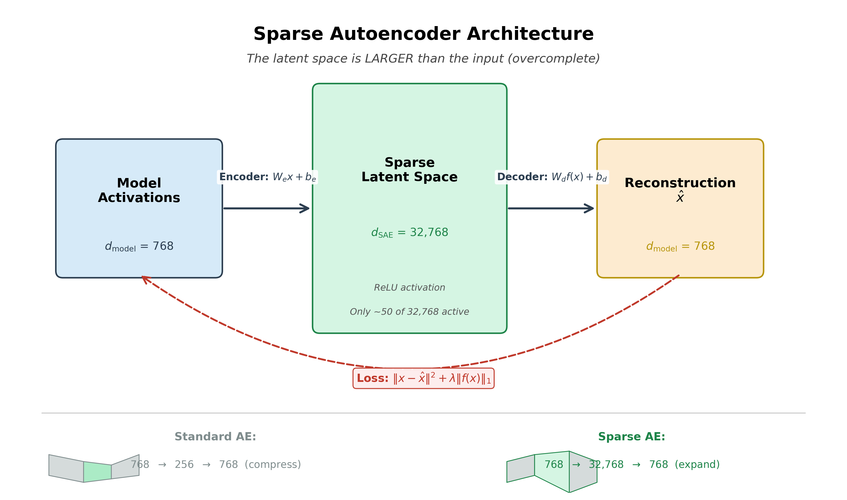
A sparse autoencoder has three components: an encoder that projects activations into a wider latent space, a ReLU nonlinearity that enforces sparsity, and a decoder that reconstructs the original activations.

Sparse Autoencoder (SAE): A neural network with a wider latent space trained to reconstruct model activations while keeping most latent activations zero. The encoder maps $d_{\text{model}}$ dimensions to $d_{\text{SAE}}$ dimensions, and the decoder maps the sparse code back.

The encoder projects activations from the model's dimensionality to a much larger latent space, then applies ReLU to enforce non-negativity:

\mathbf{f}(\mathbf{x}) = \text{ReLU}(\mathbf{x} W_e + b_e)

where $W_e \in \mathbb{R}^{d_{\text{model}} \times d_{\text{SAE}}}$ and $d_{\text{SAE}} \gg d_{\text{model}}$ . Typical expansion factors range from 4x to 256x. A model with 768 dimensions might use a latent space of 32,768 dimensions. The ReLU ensures that latent activations are non-negative, and most are zero, producing the sparsity we need.

The decoder projects the sparse latent representation back to the model's dimensionality:

\hat{\mathbf{x}} = \mathbf{f}(\mathbf{x}) W_d + b_d

where $W_d \in \mathbb{R}^{d_{\text{SAE}} \times d_{\text{model}}}$ . Each row of $W_d$ is a feature direction in the activation space. When a latent dimension is active, the corresponding row contributes to the reconstruction. The decoder learns the dictionary of features.This is the opposite of a standard autoencoder. A standard autoencoder compresses: 768-dimensional input becomes a 256-dimensional latent representation, then is reconstructed back to 768 dimensions. The purpose is dimensionality reduction. An SAE expands: 768-dimensional input becomes a 32,768-dimensional latent representation. The purpose is not compression but decomposition, finding many individual features that combine to form the input. The sparsity constraint ensures that only a few of those 32,768 dimensions are active for any given input.

The loss function combines two objectives that pull in opposite directions:

\mathcal{L} = \underbrace{\|\mathbf{x} - \hat{\mathbf{x}}\|_2^2}_{\text{reconstruction}} + \underbrace{\lambda \|\mathbf{f}(\mathbf{x})\|_1}_{\text{sparsity}}

The reconstruction term grows when the SAE discards information needed to reproduce the sampled activation. The L1 term penalizes the total magnitude of latent activations, encouraging many zeros. The coefficient $\lambda$ controls a tradeoff: higher values usually produce sparser codes but worse reconstruction. Sparser does not automatically mean more interpretable, so both properties need separate evaluation.

The SAE architecture: encoder projects activations to a wider latent space, ReLU enforces sparsity, decoder reconstructs — Figure 1: The sparse autoencoder architecture. The encoder projects d_model activations into a wider m-dimensional latent space with ReLU sparsity, and the decoder reconstructs the original activations.

Choosing $\lambda$ is a practical challenge. Too much sparsity can discard information or leave useful patterns unrepresented. Too little can permit dense codes that are difficult to interpret. Neither regime guarantees a particular set of ground-truth features.

Training SAEs

SAEs are trained on model activations, not raw text. The process works as follows:

Run the target model on a large corpus of text.
Collect the activations at a chosen site (for example, the residual stream at layer 6) for every token.
Use these collected activations as training data for the SAE.

The SAE trains on activation vectors rather than directly on text tokens. Each batch is encoded, sparsified, decoded, and scored by the reconstruction-plus-sparsity loss. The target model's weights remain frozen; the SAE is a separate learned decomposition, not a modification of the target model's normal forward pass.The microscope analogy is useful only up to a point. A physical lens does not learn what to display, while an SAE's training objective and hyperparameters determine its decomposition. Treat its latents as hypotheses about structure, not passive observations.

Expansion factor, activation site, and training-data coverage all change the dictionary an SAE learns:

Expansion factor: How many latent dimensions relative to the input. Larger expansion means more potential features but also more dead features (latent dimensions that never activate) and higher compute cost.
Where to apply the SAE: A residual stream, MLP output, or attention output presents a different activation distribution and a different interpretive question. Results from one site should not be assumed to describe another.
Training data volume: Bricken et al. trained on 8 billion activations [2]. Rare features (such as legal citations or DNA sequences) require enormous numbers of tokens before they appear in enough training examples.

Pause and think: Standard autoencoders vs. sparse autoencoders

A standard autoencoder compresses a 768-dimensional input into a 256-dimensional latent space and reconstructs back to 768 dimensions. An SAE expands a 768-dimensional input into a 32,768-dimensional latent space and reconstructs back to 768 dimensions. Both minimize reconstruction error.

Why does the SAE need a sparsity penalty while the standard autoencoder does not? What would happen if you trained an SAE without the L1 term? Consider what constraint forces a standard autoencoder to learn useful structure (the bottleneck), and what plays the analogous role in an SAE.

Towards Monosemanticity: Results

Bricken et al. applied their SAE to a one-layer transformer with a 512-neuron MLP layer [3]. The SAE had a 16x expansion factor: 512 MLP neurons became 8,192 latent dimensions. Trained on 8 billion activations collected from the model processing diverse text, the central question was straightforward: can the SAE decompose 512 polysemantic neurons into clean, monosemantic features?

The trained SAE yielded the following headline count:

512 \text{ neurons} \longrightarrow 4{,}000+ \text{ interpretable features}

Many inspected latents admitted concise labels, including Arabic script, DNA sequences, legal language, HTTP requests, Hebrew text, and nutrition statements. The SAE produced roughly eight times as many live, interpretable latents as the original layer had neurons. This is consistent with the superposition picture, but the experiment does not establish a one-to-one match between SAE latents and the model's unique “true features.”

Human raters judged approximately 70% of a large random sample of SAE latents interpretable under the study's rubric, compared with much lower scores for individual neurons [4]. That is evidence that the SAE produced more labelable units in this setting, not that every label was complete or causally correct. Some latents remained polysemantic, especially in smaller dictionaries, while larger dictionaries produced cleaner examples in the reported comparison.Concurrent work by Cunningham et al. (2023), published at ICLR 2024, also extracted interpretable SAE latents from language models. Results across research groups and model families reduce the chance that the basic phenomenon is unique to one setup, although they do not establish that SAEs recover a model's one true feature decomposition.

Bricken et al. provided four distinct lines of evidence for the quality of their features:

Detailed case studies: In-depth investigation of specific features, constructing computational proxies to verify their function.
Human evaluation: Raters assessed a large random sample, finding the 70% interpretability rate described above.
Automated interpretability (activations): LLMs generated descriptions from activation patterns, then tested those descriptions on held-out data.
Automated interpretability (logit weights): Analysis of how features influence the model's output distribution.

The methods answer complementary questions. Detailed case studies examine individual latents closely; human evaluation estimates how often people can assign coherent labels under a rubric; and automated methods scale predictive description tests to thousands of latents. Agreement across them is stronger evidence than any one score, but it still does not uniquely identify the model's computational units.

The results show that an SAE can replace a difficult neuron basis with a much sparser basis containing many human-interpretable latents, at least in this small model. Whether those latents faithfully recover the model's own computational units is a stronger question, taken up in the later article on SAE evaluation.

For how researchers inspect and interpret the features SAEs discover, including the feature dashboard methodology and automated interpretability at scale, see the next article on feature dashboards and automated interpretability. For the question of whether this approach scales to production-size models, see scaling monosemanticity.