Training Models to Be Interpretable

Interpretability as a Training Constraint

Every technique in this curriculum so far has taken the model as given. Someone else trained it, we arrive afterwards, and we go looking for structure. Probes, SAEs, attribution graphs, the parameter decomposition of the previous two articles: all post hoc, all working against a model that was optimized for loss alone and owes us nothing.

They all run into superposition. A dense network represents more features than it has dimensions, so neurons are polysemantic, and every decomposition method is in some sense trying to undo a compression the network performed during training [1]Toy Models of Superposition
Elhage, N., Hume, T., Olsson, C., et al.
Anthropic, 2022. On the standard reading, a dense model approximates the computations of a much larger, untangled, sparse network. Rather than recover that untangled network from the compressed one, train it directly [2]Weight-Sparse Transformers Have Interpretable Circuits
Gao, L., Rajaram, A., Coxon, J., Govande, S. V., Baker, B., Mossing, D.
arXiv, 2025.

Forcing Most Weights to Zero

Force the vast majority of weights to be exactly zero. Not activations, and not experts: the weights themselves, so that each neuron has only a handful of connections. In the sparsest models roughly 1 in 1000 weights is nonzero.This is the opposite of mixture-of-experts sparsity, which in this terminology is weight-dense: an MoE model's weights are almost all nonzero, it just does not use all of them on every token. Here the weights are gone.

A neuron that can only read from three residual channels cannot participate in a representation smeared across thirty of them. A model with few connections per neuron cannot afford to spend several neurons on one concept. The constraint does not forbid superposition so much as make it expensive, and the model's cheapest remaining option is to give concepts their own channels.

After each AdamW step, everything in each weight matrix is zeroed except the largest-magnitude entries, keeping the same nonzero fraction in every matrix. The target sparsity is annealed in from fully dense over training. Mild activation sparsity is applied on top, about 1 in 4 activations nonzero. The models are GPT-2-style decoder-only transformers trained on Python code.

Measuring Whether It Worked

A model counts as more interpretable here if each of its individual behaviors is implemented by a compact standalone circuit, on the reasoning that an untangled model should be easy to untangle.

A node is one neuron, one attention channel, one residual channel read, or one residual channel write -- rows and columns of weight matrices, which is as fine-grained as nodes get. An edge is a single nonzero entry in a weight matrix. There is no abstraction layer at all. The circuits are stated in the model's own coordinates rather than in a learned basis, so nothing sits between the explanation and the weights [3]Weight-Sparse Transformers Have Interpretable Circuits
Gao, L., Rajaram, A., Coxon, J., Govande, S. V., Baker, B., Mossing, D.
arXiv, 2025.

Twenty hand-built Python next-token tasks supply the behaviors, each a forced choice between two completions. One asks whether a string should close with ' or ", differing only in the opening quote. Another asks whether a variable should be followed by .add or +=, differing only in whether it was initialized to set() or "". For each task, the model is pruned to the smallest circuit reaching a target loss, with pruned nodes mean-ablated to their average activation over the pretraining distribution. The headline metric is the geometric mean edge count across tasks.

Sixteen-Fold Smaller Circuits

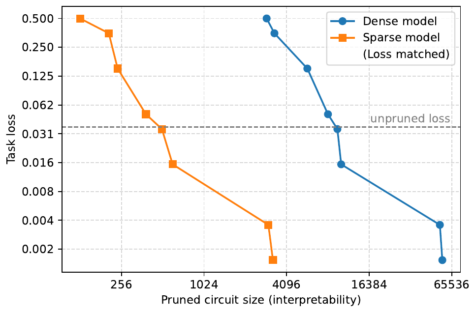
Compare a sparse model against a dense model with the same pretraining loss, and sweep the target task loss. At every accuracy level, the sparse model's minimal circuit is roughly 16 times smaller. Because the two models are matched on pretraining loss rather than on size, they are equally good at predicting text, and one of them explains itself in a sixteenth of the parts.

Mean-ablating every neuron except the few in the circuit preserves task loss, so the circuit is sufficient. Deleting just those few nodes severely harms task loss, so it is also necessary. Most published circuits establish sufficiency and leave necessity implicit, which permits a circuit that merely contains enough machinery to do the task while the model actually uses something else. Testing both is a stricter bar than most of the circuit evaluation literature meets.

The Frontier

Weight sparsity is a dial, not a setting, and turning it up costs pretraining loss.

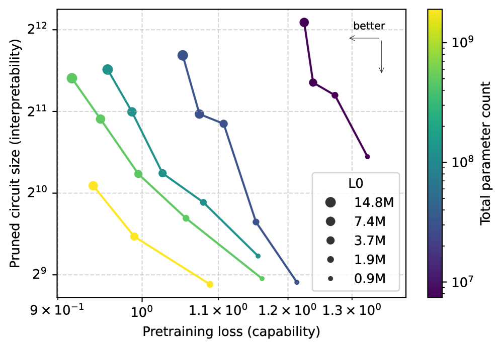
Hold total parameter count fixed and make the weights sparser: pretraining loss gets worse, circuits get smaller. That is a trade, and it is the frontier we are on. Hold sparsity fixed and make the model wider: both improve at once, and the whole frontier moves outward.

So the trade is not fundamental, only current: scale buys back what sparsity costs. A wider model at the same nonzero-weight budget is strictly more expressive and has fewer nonzero weights per neuron.There is an information-theoretic gloss on this. The number of bits needed to say which parameters are nonzero is roughly $\mathcal{O}(L_0 \log N)$ for $L_0$ nonzeros out of $N$ total, so growing $N$ at fixed $L_0$ buys additional freedom in choosing the sparsity pattern at only logarithmic cost. A related effect: increasing weight sparsity raises the sparsity of residual-stream activations on its own, without being asked to.

The models here span 0.9M to 14.8M nonzero parameters, and the authors report that pushing past tens of millions while preserving interpretability remains unsolved. The demonstrated range is narrow.

Pause and think: what does the second axis actually measure?

The vertical axis in Figure 2 is "pruned circuit size (interpretability)". Take the parenthetical seriously for a moment and ask what could go wrong with it.

Circuit size is a proxy. It measures how few parts suffice, not whether those parts mean anything. A model could in principle have very compact circuits made of nodes that each do three unrelated things, and score well here while being no easier to understand. The authors say this directly: compact task-specific circuits do not fully capture intuitive notions of interpretability, and their qualitative investigations point at a stronger notion they have not managed to codify.

This is the same problem SAE evaluation has. Sparsity and reconstruction are measurable; interpretability is what we want; and the gap between them is where a metric can be gamed. The difference here is that the metric is defined on the model's own weights rather than on a learned dictionary, so at least there is no additional layer in which the gaming could hide.

A Circuit With Nothing Left Out

The quantitative results say circuits are small. Whether small means understandable is a separate question, and the only way to answer it is to read one. Three were read manually, across two models, at roughly a researcher-day each.

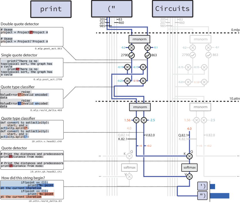
A string opens with either ' or " and must close with the matching one. The circuit that does it has 12 nodes and 9 edges, and Figure 3 omits nothing.

The layer-0 MLP has one neuron that fires on an opening double quote and another that fires on an opening single quote; between them they produce two residual channels, one positive on both quote types and one whose sign distinguishes them. Call these the quote detector and the quote type classifier. Then a single attention head in layer 10 reads the detector as a key and the classifier as a value, with a constant positive query, so the final position attends to wherever a quote was opened and copies the sign of the classifier forward. Positive means double, negative means single.

The mechanism is not a summary or an abstraction: those are the actual weights, and the numbers on the edges are the actual numbers. It is also small enough to hold in your head, which is a property no feature-level attribution graph of a frontier model has.

The circuit's four main components have 41 edges connecting them to the rest of the network, of which this circuit uses 9. If components generally have so few total edges, it might eventually be possible to trace circuits by inspecting the weights alone, with no task-specific dataset at all -- though this remains a hope rather than a finding. The other two circuits are less encouraging on this point. Bracket counting used 6 channels carrying 283 edges between them, plus another 1,217 from components elided from the write-up, and the authors judge that tracing it without task-specific data would likely be difficult.

Understanding That Predicts a Failure

A circuit read off the weights can be complete, validated, and still tell us nothing we could not have got from a behavioral description. The bracket-counting circuit went further: it predicted a way to break the model that nobody had tried.

The task is closing a flat list with ] versus a nested list with ]]. The embedding of [ writes to a few residual channels that act as open-bracket detectors. A layer-2 attention head has a near-zero query and constant keys, so its softmax is uniform and the head simply averages the open-bracket detector over the whole context, writing the result to one residual channel whose magnitude encodes nesting depth. A layer-4 head then thresholds that magnitude by using it as a query against a strong attention sink: below the sink logit nothing happens, above it the head writes a "close with two brackets" signal.

Depth is stored as a mean over the context, and a mean shrinks as the context grows, so padding the context should dilute the signal. That prediction comes out of the circuit rather than out of testing, and both attacks it suggests work: unmatched open brackets in a preceding comment fool the model into ]] on a flat list, and a sufficiently long nested list makes it predict ] instead of ]], with the error tracking the magnitude of that one residual channel as $1/n_{\text{ctx}}$ would predict.

The attack then transfers to dense models of comparable capability, so the mechanism was not an artifact of sparse training. Something similar is happening in the dense model, where it would have been much harder to find.

Pause and think: what would follow if the attack had not transferred?

We would still have a complete, validated, human-readable circuit, and a novel adversarial example derived from it. That is a real demonstration that the method produces genuine understanding of the model it was applied to.

But the objection to this whole research direction is that weight-sparse models are a different kind of object. They are trained under a constraint no useful model is trained under, at 100 to 1000 times the compute of a dense model of equal capability, and they will never be frontier systems. If their circuits are idiosyncratic to sparse training, the understanding does not travel and the models are a dead end.

Transfer is the evidence against that. The dilution attack was derived from a mechanism read off sparse weights and it breaks dense models too, which is weak but direct support for the assumption the whole program rests on: that transformers learn recurring circuit motifs, and that seeing them clearly in a sparse model tells you what to look for elsewhere. The authors also report that the tokens which are hard and easy for their sparse models are largely the same ones that are hard and easy for dense models.

Bridges to Dense Models

The dilution attack transferred because a sparse and a dense model happened to compute the same way, which is an argument from resemblance. A tighter link would tie a sparse model to one specific dense model by construction, and there is a preliminary attempt at that.

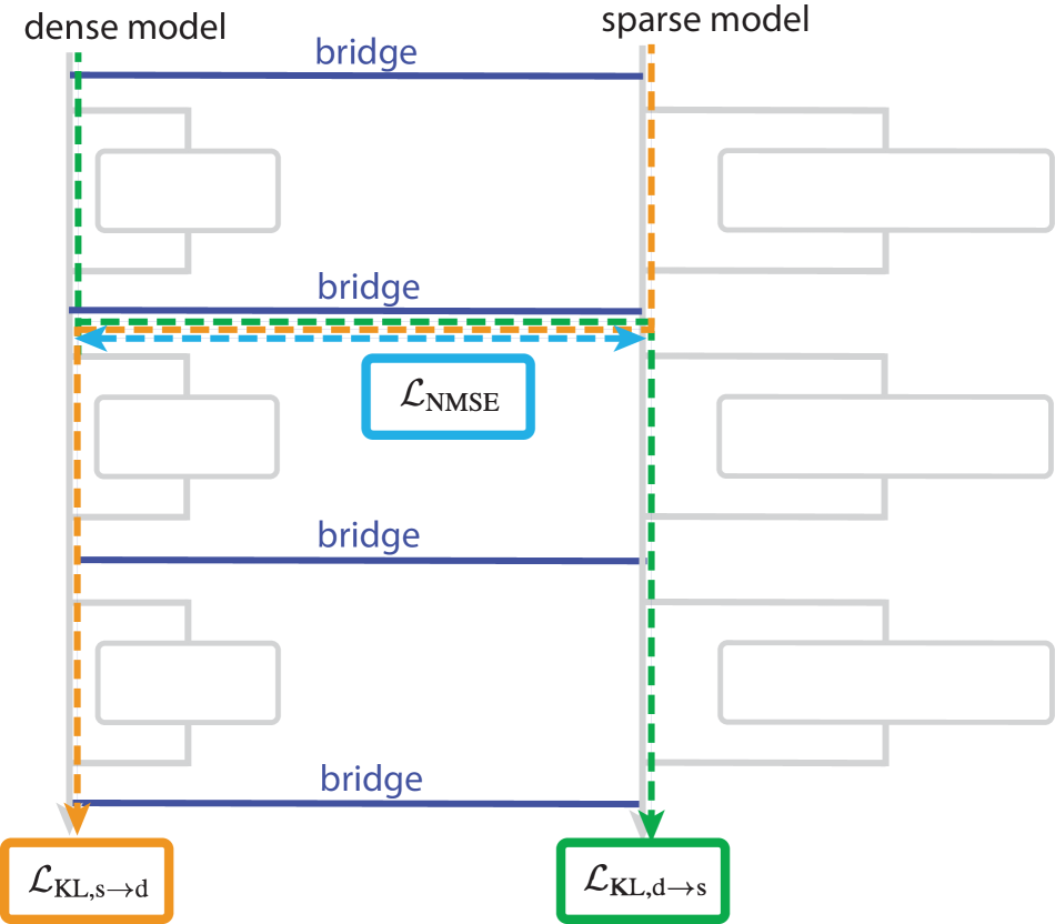
Train a weight-sparse model alongside an existing dense model, with a bridge at each sublayer: an encoder mapping dense activations to sparse ones and a decoder mapping back.Each bridge is effectively a sparse autoencoder whose latent space is another model's residual stream, with an AbsTopK encoder and a linear decoder. The unusual part is that the latents are not learned features but the activations of a second network that is being trained at the same time. Beyond the usual pretraining loss, the objective includes a normalized MSE term training each encoder to predict sparse activations from dense ones and vice versa, plus KL terms on hybrid forward passes that convert between the two activation types at a single location and require the result to still match the dense model.

A perturbation found in the interpretable model can then be pushed into the uninterpretable one. Pick a node from a pruned sparse circuit that both matters for the task and encodes something recognizable, perturb it in the sparse model, and map the perturbation through the bridge.

Steering the sparse model's quote type classifier from its double-quote value toward its single-quote value, then bridging, sharply raises the dense model's probability of emitting a single quote. In a second task, a channel that goes strongly negative on lines beginning if, while, or except -- lines that must end in a colon -- is steered from its return True value toward its while True value, and the dense model's probability of a colon rather than a newline goes up, though less sharply.

Both are preliminary and the authors label them so. But the perturbation applied to the dense model was chosen by reading a circuit in the sparse one, which is not something post-hoc analysis of the dense model alone would have supplied.

Are Individual Weights Interpretable?

The circuits above were found behavior-first: pick a task, prune, read. That approach cannot say anything about a weight that participates in no task you thought to test, and a weight can serve different functions on different parts of the input distribution.

A follow-up asks the inverted question, on the same models: can we say what an individual weight does across the whole training distribution, without choosing a behavior first [8]Individual Parameters in Weight-Sparse Transformers Appear Interpretable
Marin-Llobet, A., Heimersheim, S.
arXiv, 2026? A weight counts as explained, in their sense, if we can say when it matters -- on which inputs ablating it changes the model's predictions.

The pipeline is automated end to end. Ablate one weight, measure per-position KL divergence against the unablated model across a corpus, take the token contexts accounting for the top 90% of cumulative KL, and hand them to an LLM with instructions to return a Python predicate f(tokens, pos) -> bool describing what they have in common. Then score the predicate causally. Ablate the weight everywhere, restore it only where the predicate fires, and measure how much of the ablation's effect on cross-entropy that recovers; separately, restore it only where the predicate does not fire, which guards against a predicate that succeeds by being vacuously broad. A coverage cap rules out predicates that fire nearly everywhere. Best of 100 candidates, and the weight counts as interpretable only if its best predicate clears the threshold on held-out text.

Pooled across sampled nonzero weights, the score is 15% for the weight-sparse code transformer, 9.6% for a sparse SimpleStories model, 1.5% for its dense counterpart, and 0.4% for Pythia-70m. Restricting to weights whose ablation actually does something -- high cross-entropy impact -- the sparse models reach 20 to 30% against 0 to 3% for the dense controls, and the paper's headline range is that 12 to 31% of weights admit a single short description that identifies what the weight is for.

A sparse model's zero weights are trivially interpretable, since they do nothing, so most of a weight-sparse model's parameters have per-weight accounts available. The same is not remotely true of a dense model. Parameter decomposition learns a basis in which weights become interpretable; weight sparsity aims to make the raw weight basis interpretable directly, so no decomposition step is needed and no question arises about whether the learned basis reflects the model or the decomposition objective.

What This Costs

Unstructured weight-sparse networks need on the order of 100 to 1000 times the training and inference compute of a dense network of comparable capability, and for fundamental reasons they are unlikely to close that gap. Fully interpreting a frontier model this way, or training an interpretable frontier model from scratch, is not going to happen.

Circuits for the more complex tasks contain polysemantic nodes, with concepts still smeared across several of them, far less than in a dense model but not eliminated. Features are not all binarizable, so some carry information in their magnitude and explaining them means explaining the magnitude too -- the bracket-depth channel is exactly this. Mean ablation is an imperfect faithfulness test, and full confidence would need something like causal scrubbing [9]Causal Scrubbing: A Method for Rigorously Testing Interpretability Hypotheses
Chan, L., Garriga-Alonso, A., Goldowsky-Dill, N., et al.
Redwood Research, 2022. The pruning algorithm prunes nodes rather than edges and leaves residue that has to be cleared by hand. And weight sparsity may not be the only inductive bias needed; expert sparsity is floated as a complementary one.

Whether fine-grained explanation scales at all is a worry that goes beyond weight sparsity. Even optimistically, applying this method to complex behaviors in capable models would produce enormous circuits, because the explanations are maximally fine-grained, and making sense of those may be a job for automated interpretability. Pessimistically, capable models may perform complex tasks in ways that resist simple description at all. That would put a ceiling on ambitious mechanistic interpretability as a whole.

Where This Could Go

Frontier-scale interpretable pretraining is off the table, so the proposals aim lower.

Scale the sparse models into a series of interpretable model organisms, up to something like GPT-3 capability, on the bet that transformers learn universal circuit motifs and that seeing them clearly at small scale tells you what to look for at large scale. Bridged sparse models would make this sharper, since comparing a sparse model's computations against a dense one's is a way to study superposition and interference weights in the dense model directly.

Or spend the compute on understanding less. Train a bridged sparse model on a narrow but important task distribution -- deception, refusal, goal-seeking -- rather than a whole pretraining corpus. That would not reverse-engineer a frontier model, but it could support a safety case about a specific behavior, which is a more modest and more achievable target.

Or treat sparse circuits as primitives for automated interpretability. Dictionary learning gave the field a language in which computations are simpler to state, and sparse circuits give another; if automation is bottlenecked on primitives rather than on the automation itself, better primitives are what unblocks it.

Looking Ahead

Both halves of this block push against an assumption the rest of the curriculum shares, that interpretability is something applied to a model after the fact. Parameter decomposition keeps the model and changes the coordinates; weight-sparse training changes the model. Neither has been demonstrated near frontier scale, and both are honest about it.

The next block turns to what interpretability is for. Many of the arguments there assume we can locate a behavior in a model we did not train, using methods whose faithfulness is contested -- a tension the limitations article takes up directly. The work here is one response to that tension: if the mechanisms we need are not legible in models as they are built, perhaps the models should be built differently.