The Superposition Hypothesis

The Fundamental Tension

In earlier articles on circuit analysis, features aligned neatly with individual attention heads. A Name Mover head moved names. An S-Inhibition head suppressed repeated subjects. Each component had one clear role, and we could study the model one head at a time. But what happens when features do not align with heads, when a single head participates in multiple unrelated computations, and a single feature is distributed across many components?

Mixed and distributed representations are common enough that a one-component, one-concept assumption needs evidence rather than being a safe default.

Why neurons can be polysemantic. Early vision interpretability work found neurons that responded to both wolves and Coca-Cola cans. One explanation is that features which rarely co-occur can share representational capacity at little cost. A “wolf neuron” label based only on wolf images would then capture one real response while hiding another.

The same phenomenon appears in language models. A neuron might fire for "baseball" and "academic citations." A head might participate in five different circuits for five different tasks. The clean one-to-one mapping between components and concepts that would make interpretability easy simply does not exist in most models.

The reason is a counting problem at the heart of neural network representations.

Consider a language model with a residual stream of dimension $d = 512$. If each feature gets its own orthogonal direction, the model can represent at most 512 features. But language understanding requires far more than 512 features. The model needs to track syntax, semantics, entities, relationships, sentiment, factual knowledge, and more. There are plausibly millions of features that a model would benefit from representing.The term 'feature' here means any property of the input that the model finds useful for prediction. A feature might be 'this token is a proper noun,' 'the sentence is a question,' 'the subject is plural,' or 'the text is discussing sports.' Features range from simple syntactic properties to complex semantic and factual associations.

The fundamental tension is stark:

$$\text{Features the model wants} \gg \text{Dimensions available}$$

A 512-dimensional residual stream has 512 orthogonal directions. But the model might need to represent 10,000 or 100,000 distinct features. What does the model do?

Two limiting strategies make the tradeoff clear. A model could allocate orthogonal directions to a subset of features and omit the rest, avoiding cross-feature interference among those it retains. Or it could use non-orthogonal directions to represent more features while accepting some interference. Trained toy models can mix these strategies, dedicating dimensions to important dense features and superposing sparser ones.

Superposition: A neural network exhibits superposition when it represents more features than it has dimensions using non-orthogonal feature directions. Because the directions overlap, a readout for one feature can receive interference from others.

In the toy-model framework, superposition emerges from optimizing reconstruction rather than being built into the architecture [1]Toy Models of Superposition
Elhage, N., Hume, T., Olsson, C., et al.
Anthropic, 2022. Feature importance and sparsity help determine which solution is economical: errors on important features cost more, while rarely co-active features interfere less often. Real transformers add many complications, so the toy result is a proposed explanatory mechanism rather than a proof that every mixed representation has this cause.

Where Superposition Lives: Privileged and Non-Privileged Bases

Before we study superposition in a toy model, we need to understand a subtlety that changes where and how superposition manifests. Not all activation spaces in a transformer are created equal. The difference comes down to whether the nonlinearity treats each dimension individually.

Why ReLU creates a privileged basis. In an MLP, a vector enters the hidden layer, gets multiplied by $W_{\text{in}}$ to produce a pre-activation vector, and then ReLU zeroes out the negatives independently for each dimension. This elementwise operation makes each axis special. Suppose the hidden layer is 3-dimensional and the pre-activation is $[2.1, -0.4, 0.7]$. ReLU produces $[2.1, 0, 0.7]$: neuron 1 is "on," neuron 2 is "off," neuron 3 is "on." Each neuron has its own gate. The nonlinearity treats the axes individually, so the axes are the natural units of analysis.

Privileged basis: An activation space has a privileged basis when the model's computation treats each coordinate axis differently, typically because a nonlinear activation function (like ReLU or GELU) is applied elementwise. In a privileged basis, individual dimensions (neurons) are meaningful units of analysis.

Why residual coordinates are less privileged. Attention and MLP blocks enter and leave the residual stream through learned linear maps. If we ignore operations that explicitly depend on residual coordinates, we can rotate the residual basis by $R$ and compensate in every reading and writing matrix. A query projection, for example, becomes $(\mathbf{r}R)(R^{-1}W_Q)=\mathbf{r}W_Q$. This reparameterization changes individual coordinates without changing the function. Layer normalization, learned per-coordinate scales, and some architectural details restrict the exact symmetry, but a raw residual coordinate is still much less naturally distinguished than a post-activation MLP neuron.

Non-privileged basis: An activation space has a non-privileged basis to the extent that coordinated changes of basis can leave the model's function unchanged. Individual coordinates then have no architecture-independent interpretation.

Pause and think: Does rotating the MLP hidden layer preserve computation?

Consider an MLP hidden layer with ReLU activation. If you rotate the hidden layer activations by an orthogonal matrix $R$, does the MLP compute the same function? Think about what ReLU does to a rotated vector versus the original.

It does not. ReLU applied to $\mathbf{x}R$ is not the same as $\text{ReLU}(\mathbf{x})R$. Rotation mixes dimensions, and then ReLU zeroes out different entries than it would have in the original basis. For example, if $\mathbf{x} = [1, -1]$ and $R$ is a 45-degree rotation, $\text{ReLU}(\mathbf{x}) = [1, 0]$ but $\text{ReLU}(\mathbf{x}R) = \text{ReLU}([1.41, 0]) = [1.41, 0]$, which gives a different result when rotated back. The elementwise nonlinearity breaks rotation invariance, creating the privileged basis.

This distinction produces two flavors of superposition with different consequences:

• MLP hidden layers have a privileged basis. Individual neurons are meaningful units, but each one may serve multiple roles. Neuron 42 fires for "sports" and "the color red." We can see individual neurons, but they are not monosemantic. This is computational superposition: the right units of analysis are clear (neurons), but each unit is overloaded.
• The residual stream has a much weaker coordinate privilege. Features are usually studied as directions or subspaces rather than by assigning intrinsic meaning to “dimension 42.” This is representational superposition: the useful units need not coincide with the stored coordinate basis.

The practical consequences are direct. When MI researchers say "neuron 42 in layer 6 fires for X," they are relying on the privileged basis: each neuron has its own activation gate that makes it individually meaningful. When they say "there is a direction in the residual stream that encodes sentiment," they cannot point to any single dimension because the residual stream has no privileged basis. This is also why sparse autoencoders behave differently depending on where they are trained: applied to the MLP hidden layer, an SAE decomposes neurons into finer-grained features; applied to the residual stream, it decomposes the whole space into features, since there are no natural units to start from.

The Toy Model

To study superposition systematically, Elhage et al. built a toy model that isolates the core question: given $m$ features and $n < m$ dimensions, how does the network allocate directions? [2]Toy Models of Superposition
Elhage, N., Hume, T., Olsson, C., et al.
Anthropic, 2022

The architecture is deliberately simple. The input is a nonnegative vector $\mathbf{x} \in \mathbb{R}^m$ with $m$ features, each with known importance and sparsity. A linear map compresses it to an $n$-dimensional hidden representation, and a decoder followed by ReLU reconstructs the original features:

$$\mathbf{h}=\mathbf{x}W_e, \qquad \hat{\mathbf{x}}=\text{ReLU}(\mathbf{h}W_d+\mathbf{b})$$

The original tied-weight version uses $W_d=W_e^\top$. ReLU is applied to the reconstructed features because the synthetic features themselves are nonnegative; the $n$-dimensional bottleneck is linear.

Why a toy model? Real transformers are too complex to isolate superposition cleanly. The toy model gives us direct control over two experimental knobs. Feature importance $I_i$ controls how much each feature matters for reconstruction: errors on a high-importance feature cost more. Feature sparsity $S_i$ controls how often each feature is active: high sparsity ($S_i \approx 1$) means it is almost always absent. Because $n$ is small (2D or 3D), we can visualize the learned representations directly.

The model minimizes weighted reconstruction error:

$$\mathcal{L} = \sum_{i=1}^{m} I_i \cdot \mathbb{E}[(x_i - \hat{x}_i)^2]$$

where $I_i$ is the importance of feature $i$ and the expectation is over the data distribution, which determines how often each feature is active. This setup lets us ask precisely: given these importances and sparsities, does the trained model use superposition?

Phase Diagrams

Elhage et al. trained many toy models, varying feature importance and sparsity systematically [3]Toy Models of Superposition
Elhage, N., Hume, T., Olsson, C., et al.
Anthropic, 2022. For each model, they measured whether the learned representation used superposition (non-orthogonal feature directions) or dedicated dimensions (orthogonal directions). The result is a phase diagram: a map showing where in the importance-sparsity space superposition occurs.

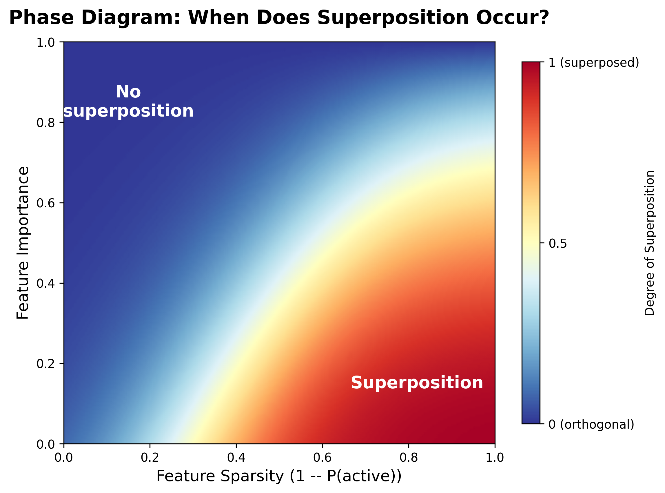
The phase diagram has two clear regions. The blue region (high importance, low sparsity) shows no superposition, features get their own orthogonal dimensions. The red region (low importance, high sparsity) shows strong superposition, features are packed into shared dimensions. The transition between regions is sharp, like a phase transition in physics.

Why does importance matter? Interference on a high-importance feature is expensive, so the model has a stronger incentive to dedicate an orthogonal dimension to it. A low-importance feature can tolerate more reconstruction error and is therefore a better candidate for a superposed representation.

Sparsity makes superposition economical. Two dense features interfere constantly, but two sparse features rarely co-occur. They interfere only when both are active simultaneously:

$$P(A\text{ and }B\text{ active}) = P(A\text{ active})P(B\text{ active})$$

for independent features. If both activate on 1% of examples independently, they co-activate on 0.01%. Correlated features can collide much more often, so sparsity alone does not determine the cost.

Sparse, weakly correlated features can make superposition cheaper because the model pays the largest interference cost on fewer inputs.

In the toy model, the transition between "no superposition" and "superposition" can be abrupt as sparsity crosses a threshold. The change resembles a phase transition in physics, such as a magnet losing its magnetization above the Curie temperature. The threshold depends on feature importance, with less important features entering superposition sooner.

The toy model predicts that real language models should use superposition wherever useful features are sparse relative to the available dimensions. Many linguistic and factual properties plausibly meet that condition, and widespread polysemanticity is consistent with the prediction. The toy model does not tell us exactly how many features a language model has or place each one on its phase diagram.

The Geometry of Superposition

In the toy model, each feature $i$ is represented by a direction $\mathbf{f}_i$ in the $n$-dimensional hidden space. The encoder maps feature $i$ to direction $\mathbf{f}_i$, and the decoder reads out feature $i$ by projecting onto $\mathbf{f}_i$. The geometry of superposition is the geometry of how these directions are arranged in space.

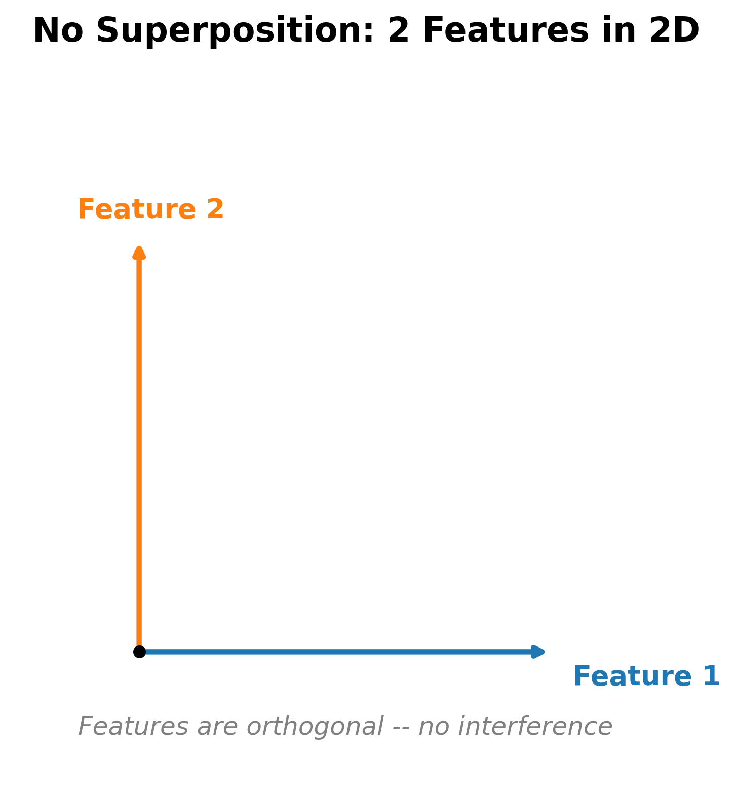
When $m = n$ (as many features as dimensions), each feature gets its own axis. The directions are orthogonal: $\mathbf{f}_i \cdot \mathbf{f}_j = 0$ for $i \neq j$. No interference, activating feature $i$ has zero effect on the readout of feature $j$. This is the ideal case.

When $m > n$, you cannot fit $m$ orthogonal vectors in $n$ dimensions. The model must use non-orthogonal directions, and the angle between feature directions shrinks below 90 degrees. The interference between features $i$ and $j$ is proportional to their dot product: $\text{interference}(i, j) = \mathbf{f}_i \cdot \mathbf{f}_j$. Orthogonal features have zero interference; parallel features have maximal interference.

Pause and think: Optimal packing in 2D

Before looking at the specific arrangements the model discovers, think about this: if you had to place 3 unit vectors in a 2D plane to minimize the maximum dot product between any pair, where would you put them? What about 5 vectors? What about $m$ vectors in general?

The toy model discovers specific geometric arrangements that minimize interference, and these depend on the ratio $m / n$. Let us walk through the progression.

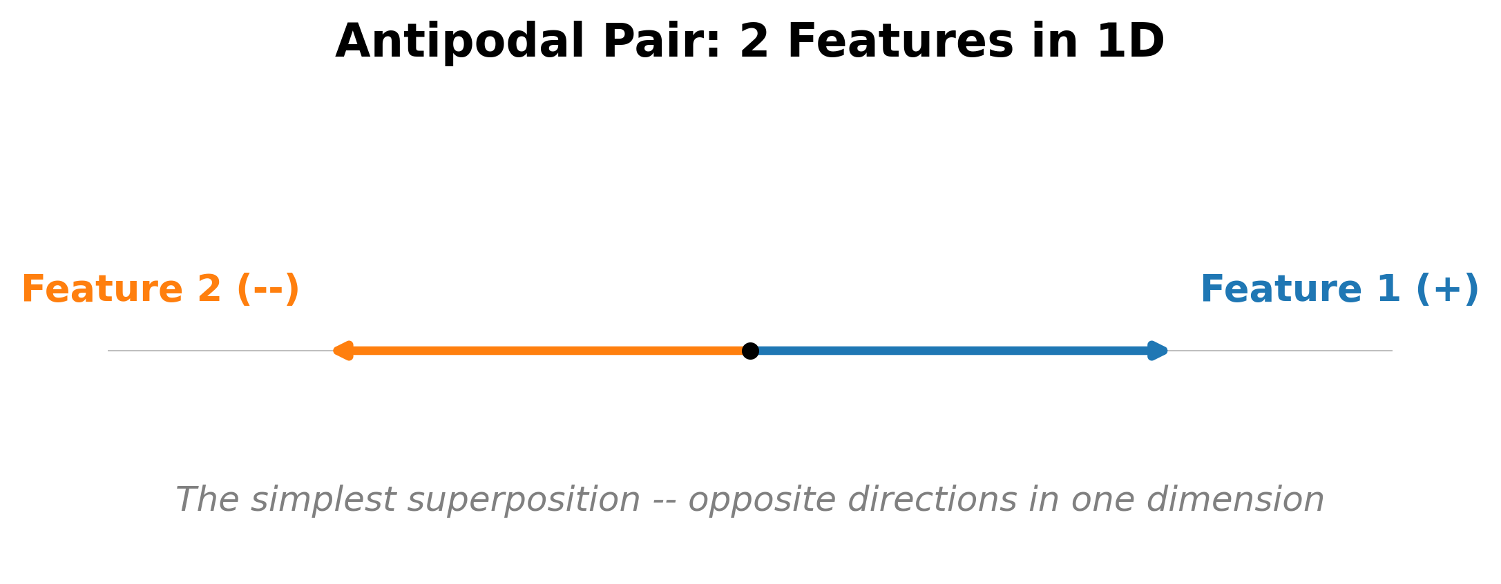
The simplest case of superposition is 2 features in 1 dimension. Feature 1 points right (+1) and feature 2 points left (-1). The dot product is $\mathbf{f}_1 \cdot \mathbf{f}_2 = -1$, which is maximally interfering. But if both features are sparse, they rarely co-occur. When only one is active, the sign tells you which one. The gamble: with high sparsity, the "both active" case is rare enough that the model comes out ahead.

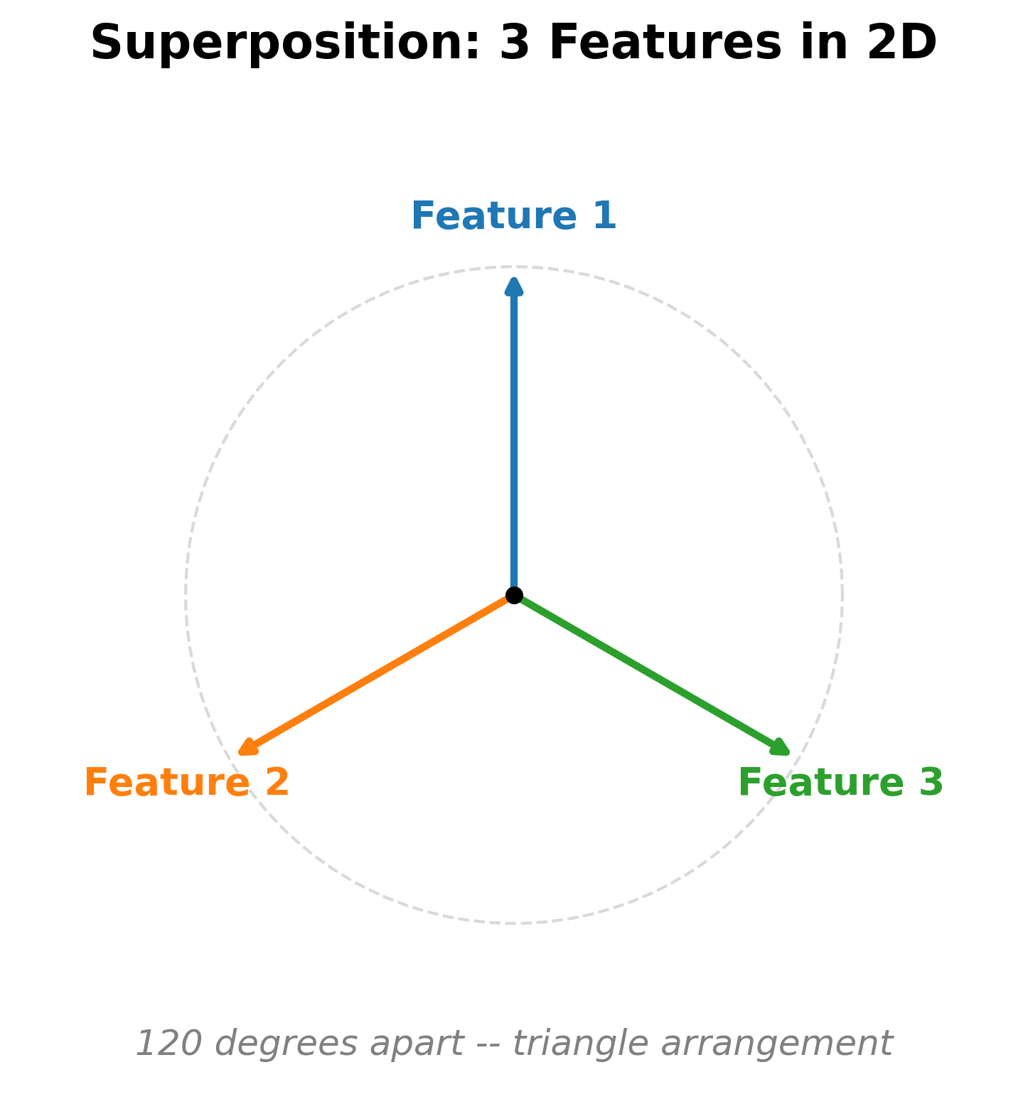
With 3 equal-importance features in 2 dimensions, one toy-model solution places three arrows 120 degrees apart, forming a triangle. The dot product between each pair is $\mathbf{f}_i \cdot \mathbf{f}_j = -0.5$. Because feature activations are nonnegative, anti-alignment behaves differently from positive overlap; the ReLU decoder can suppress some resulting cross-talk.

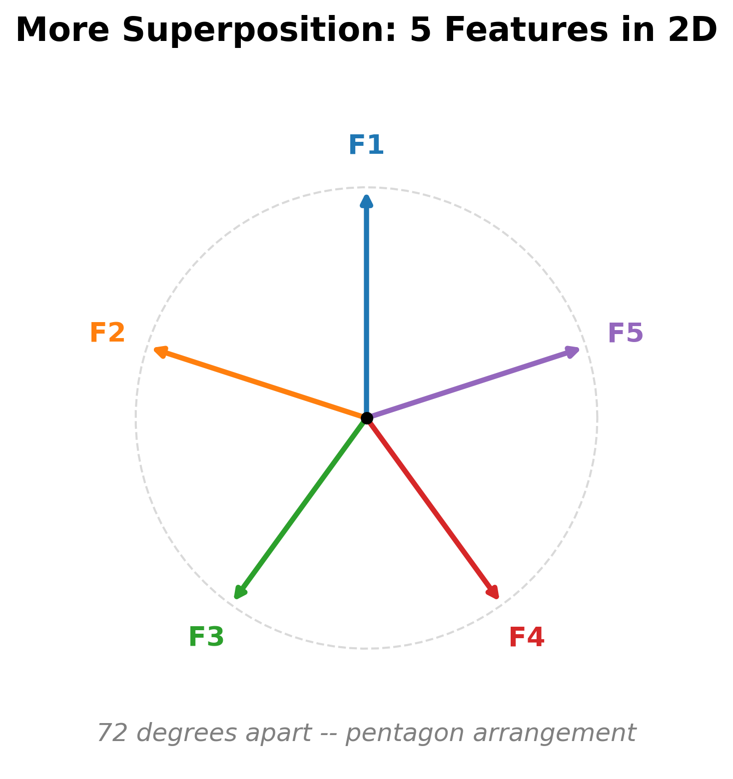
With 5 equal-importance features in 2 dimensions, a regular-pentagon solution places the directions 72 degrees apart. Adjacent features have $\mathbf{f}_i \cdot \mathbf{f}_{i+1} \approx 0.31$, while non-adjacent features have $\mathbf{f}_i \cdot \mathbf{f}_{i+2} \approx -0.81$. The positive overlap creates interference when neighboring features co-activate, so this solution becomes more attractive as co-activation becomes rarer.

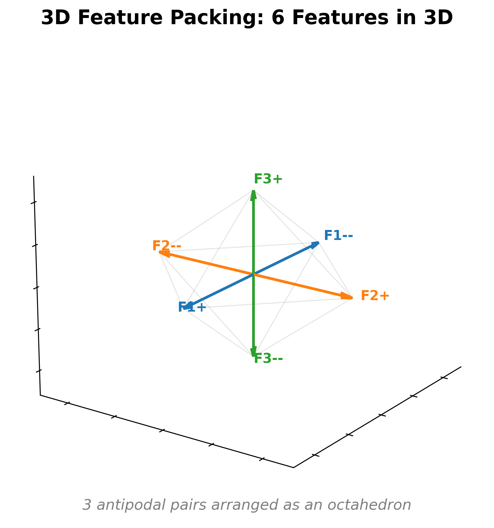
In three dimensions, the model packs 6 features as three antipodal pairs along the x, y, and z axes, forming an octahedron. Opposite features have dot product $-1$, while adjacent features have dot product $0$. The arrangement combines antipodal pairing with orthogonality.

Across symmetric toy-model settings, learned directions often resemble regular geometric arrangements: a line segment in 1D, polygons in 2D, and polyhedra in 3D.This resemblance connects the toy solutions to spherical-code and packing problems. The exact optimum still depends on the model's loss, feature probabilities, importances, nonlinearity, and whether direction signs are equivalent. Geometry provides intuition, not a universal closed-form solution. The regularity makes the tradeoff visible: spread directions to reduce harmful overlap while fitting more of them into a fixed space.

The interference grows with packing density. At low packing ratios ($m / n$ small), features are nearly orthogonal and readouts are clean. At high packing ratios ($m / n$ large), features are far from orthogonal and readouts are noisy. The model chooses the packing density that optimizes the tradeoff between representing more features and suffering more interference.

Pause and think: Geometry at scale

The toy model with 5 features in 2D discovers the pentagon arrangement. In a real transformer with $d = 768$ and potentially millions of features, what kind of geometric structure would you expect? Would the features form recognizable polytopes, or something less structured? Consider that in 768 dimensions, there is an enormous amount of room for nearly-orthogonal directions, far more than our low-dimensional intuitions suggest.

Interference and Its Cost

When features are superposed, activating one feature partially activates others. Suppose features 1 and 2 have $\mathbf{f}_1 \cdot \mathbf{f}_2 = 0.3$. When feature 1 is active with value $x_1 = 1$, the readout of feature 2 picks up a ghost signal:

$$\text{Readout of feature 2} = \mathbf{f}_2 \cdot (x_1 \cdot \mathbf{f}_1) = 0.3$$

Feature 2 "sees" a ghost activation of 0.3 even though it is not active. This is interference, and it corrupts downstream computation in two ways. False positives occur when a feature appears active when it is not, a ghost activation triggers behavior that should not have been triggered. Magnitude distortion occurs when a feature's true activation is shifted by interference from other active features, so even when a feature is correctly identified as active, its strength is wrong.

The expected cost of interference between features $i$ and $j$ depends on how often they are simultaneously active:

$$\mathbb{E}[\text{interference cost}] \propto (\mathbf{f}_i \cdot \mathbf{f}_j)^2 \cdot P(x_i \neq 0) \cdot P(x_j \neq 0)$$

The geometric interference $(\mathbf{f}_i \cdot \mathbf{f}_j)^2$ is fixed by the arrangement, but its expected cost is scaled by co-occurrence. If two independent features are each active with probability $0.01$, they co-occur with probability $0.0001$, ten thousand times less often than features that are always active.Under the toy model's independence assumptions, reducing each feature's activation probability by a factor of ten reduces their co-occurrence probability by a factor of one hundred. Correlated real-world features need not follow this calculation.

This is the superposition bargain. What the model gains: it represents $m \gg n$ features in $n$ dimensions, captures more structure in the data, and achieves lower loss on average. What the model pays: occasional interference when sparse features co-occur, noisy readouts for low-importance features, and activations that are harder to interpret. When features are sparse enough, the bargain is overwhelmingly favorable. The model gets to represent far more features at a cost that is negligible in expectation.

Why Superposition Makes Interpretability Hard

If features are superposed, individual neurons respond to multiple unrelated features. A single neuron might activate for "sports," "the color red," and "questions about geography" because these three features share that neuron's direction. This is polysemanticity: one neuron, many meanings. In a non-superposed model, each neuron would represent exactly one feature (monosemanticity). In a superposed model, neurons are mixtures.

Superposition makes neuron-by-neuron interpretation less reliable. In an idealized monosemantic network, neuron 42 might track proper nouns and neuron 43 verbs. Under a distributed code, each coordinate mixes contributions from several feature directions, so its top examples may not admit one complete label. This motivates searching for useful directions or subspaces rather than assuming every residual coordinate is itself a feature.

For circuit analysis, superposition means that the clean decompositions we found in earlier work become the exception rather than the rule. In a model with strong superposition, a single attention head might participate in five different circuits for five different tasks. The "Name Mover" feature might be distributed across twenty heads. Ablating one head disrupts all five circuits, not just the one we are studying. The confounds multiply.

Superposition creates a fundamental bottleneck for mechanistic interpretability. Neuron-level analysis fails because individual neurons are polysemantic mixtures, not clean features. Head-level analysis fails because individual heads participate in multiple circuits. Circuit discovery is harder because features overlap, making it difficult to isolate one circuit from another. Ablation experiments are confounded because ablating a component affects multiple features simultaneously.

How bad is it in practice? Evidence from real models suggests superposition is pervasive. Olah et al. (2020) documented polysemantic neurons in vision models, neurons responding to cat faces and car hoods [4]Zoom In: An Introduction to Circuits
Olah, C., Cammarata, N., Schubert, L., et al.
Distill, 2020. Elhage et al. (2022) showed that even small toy models exhibit strong superposition when features are sparse [5]Toy Models of Superposition
Elhage, N., Hume, T., Olsson, C., et al.
Anthropic, 2022. Sparse probing experiments on production language models have added direct confirmation: some neurons are monosemantic (e.g., language-detection neurons that fire reliably for a single language), but the majority are polysemantic mixtures. The monosemantic neurons tend to correspond to high-importance, low-sparsity features, exactly what the toy model predicts should escape superposition. Meanwhile, MLP layers appear to store factual associations in a superposed manner, with more facts than neurons and storage patterns that do not align with individual neuron axes. The vast majority of neurons in large language models do not have clean single-feature interpretations. Superposition is not an edge case. It is the default.

Superposition explains one major source of difficulty: the model's coordinate axes need not align with the features we want to study. Polysemantic neurons and overlapping circuits can then make component-level labels and ablations hard to interpret. It is not the field's only obstacle, but it motivates methods that search for better units of analysis.

One might hope that larger models (more dimensions) would reduce superposition. In part, yes: larger models can represent more features orthogonally. But larger models also learn more features. The number of useful features grows at least as fast as the model size, possibly faster. The ratio $m / n$ does not obviously shrink as models scale. Superposition may be a permanent feature of neural networks, not a problem that goes away with scale.

The natural question is: can we undo it? If features are encoded as directions in activation space, can we find those directions? Can we decompose a polysemantic neuron into its constituent monosemantic features? This is the decomposition problem, and the most promising current approach is sparse autoencoders (SAEs), separate networks trained to take a model's activations and decompose them into a sparse set of interpretable features. Whether SAEs deliver on this promise, and what their limitations are, is the subject of the next article.