What Does an LLM Actually Do?
At the highest level, a language model takes text as input and outputs a probability distribution over what token comes next. Feed it "the cat sat on the" and it assigns probabilities to possible continuations: "mat" might get 15%, "floor" 12%, "bed" 8%, and so on.The model doesn't see words directly. Text first goes through a tokenizer, which we'll discuss shortly.
The architecture that performs this computation is called a transformer [1]Attention Is All You Need
Vaswani, A., Shazeer, N., Parmar, N., et al.
NeurIPS, 2017. Modern models have changed many details, normalization, positional encoding, nonlinearities, attention variants, and training objectives among them, but the same broad pattern remains: attention and MLP blocks repeatedly update a residual stream.
Why Next-Token Prediction Might Mean Understanding
Memorization occurs, especially for repeated passages, but it does not explain successful continuation of unfamiliar text. Generalization requires reusable statistical structure: grammatical regularities, associations between entities, common formats, and strategies that apply across many passages.
Whether those patterns deserve the word understanding is a philosophical question we do not need to settle. Mechanistic interpretability starts from the more testable claim that next-token prediction requires internal computations, and asks what those computations are.
Tokenization: Text to Numbers
Neural networks operate on numbers, not strings. Before any computation, text passes through a tokenizer, which converts it into a sequence of integers called tokens.
The tokenizer is constructed before training (using compression techniques like Byte-Pair Encoding) and remains fixed. For common English words, each word typically becomes one token. For rare words, foreign text, or gibberish, the tokenizer breaks them into smaller pieces.You can explore how different models tokenize text at tools like OpenAI's tokenizer playground. It's worth getting an intuition for how common words become single tokens while rare words fragment into multiple pieces.
For example, with GPT-2's tokenizer:
- "The quick brown fox" becomes 4 tokens (one per word, with spaces attached)
- An uncommon word like "gimble" might become two tokens: "g" and "imble"
- Keyboard mashing produces many tokens, roughly one per character pair
Two tokenization details matter for interpretability work. First, most tokenizers prepend a special beginning-of-sequence (BOS) token to every input. This token appears at position 0 in every sequence, which makes it a fixed landmark. Attention heads that have nothing useful to attend to often default to the BOS position, using it as a "rest position." This produces a characteristic vertical stripe (column pattern) in attention visualizations: many positions attending to position 0. When you see this pattern, it usually does not mean the BOS token contains meaningful information. It means those heads are effectively idle on that input.Some models (like GPT-2) do not use a dedicated BOS token but exhibit the same column-pattern behavior on whatever token happens to be at position 0. The principle is the same: a fixed, predictable position serves as a default attention target.
Second, most tokenizers are sensitive to leading whitespace. The token for " cat" (with a space prefix) is a different token from "cat" (no space). In normal text, most words appear with a preceding space, so " cat" is the common form. This distinction trips up many MI experiments: if you manually construct prompts or look up token IDs, forgetting the space prefix gives you the wrong token.
For the rest of this article, we will take tokenization as a black box and focus on what happens once we have our sequence of token IDs.
The Big Picture
A decoder-only transformer processes a sequence by repeatedly applying two sublayers at every layer:
- Attention: move information between positions.
- MLP: transform information at each position.
Both sublayers write their outputs into a shared residual stream, which acts like a global scratchpad.
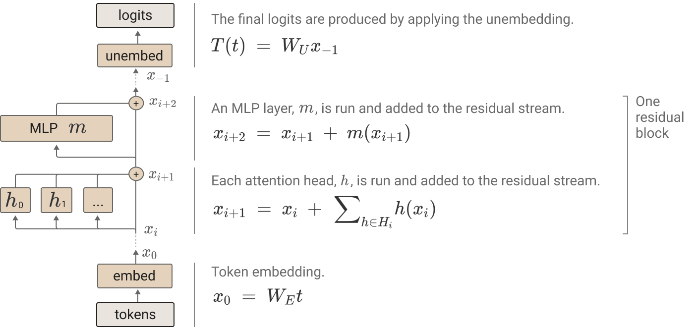
Elhage, N., Nanda, N., Olsson, C., et al.
Anthropic, 2021
Parallel Predictions
Given an input of tokens during training, the transformer can make next-token predictions in parallel. The state at position predicts token using only positions up to .This is enforced by causal masking in the attention mechanism. Position i can only attend to positions 0 through i, never to the future.
During training, a single sequence becomes training examples. Position 0 predicts token 1 given no context. Position 1 predicts token 2 given token 0. Position predicts token given all previous tokens. The model adjusts its weights to make each of these predictions slightly better.
This parallel structure is why transformers are so efficient to train compared to earlier architectures like RNNs, which had to process tokens sequentially. RNNs compute a hidden state that depends on all previous hidden states, so computing the output at position requires sequential steps. Transformers sidestep this: attention lets every position look at every earlier position in a single parallel operation. This parallelism is a major reason transformers have become dominant.
Step 0: Token Identity and Position
Once we have a sequence of token IDs, a learned lookup maps each ID to a vector in the residual stream:
The Embeddings article develops this lookup, its learned geometry, and its relationship to the output unembedding. The lookup encodes token identity but not where the token occurs.
Transformers supply order through a separate positional mechanism. Some add learned or sinusoidal vectors to . Others, including Rotary Position Embedding (RoPE), modify queries and keys inside attention, while methods such as Attention with Linear Biases (ALiBi) add distance-dependent attention biases. Positional Embeddings compares these designs and their consequences for interpretability.
Step 1: Attention (Information Routing)
Attention is the mechanism that allows tokens to communicate with each other. Each position can look at all previous positions, decide which are relevant, and gather information from them.
In self-attention, every token plays three roles simultaneously:
- Query: "What am I looking for?"
- Key: "What do I contain?"
- Value: "What information do I send if attended to?"
Each token's query is compared against every other token's key (via dot product) to produce attention weights. These weights determine how much each token contributes to the output. The final output is a weighted sum of value vectors.
Multi-head attention runs several attention heads in parallel, each with its own learned query/key/value projections. Different heads can attend to different things: one might look at the previous token, another at the subject of the sentence, another at tokens matching some learned pattern.
For the full mathematical details of attention, including the softmax normalization, scaling, and causal masking, see The Attention Mechanism.
Step 2: MLP (Local Computation)
After attention, each position passes through an MLP (multi-layer perceptron). Unlike attention, the MLP operates independently on each position: it does no cross-token communication.
Think of it this way: attention moves information between positions, then the MLP transforms the state at each position. In many common transformer designs, MLPs contain a large fraction of the non-embedding parameters. Studies also implicate them in factual recall, though knowledge is not confined to MLP weights. We cover their structure and the evidence behind the key-value-memory interpretation in MLPs in Transformers.
The Residual Stream
Residual Stream: The residual stream is the vector that flows through the transformer, updated additively by each component. Every attention head and MLP reads from it and writes to it.
The residual stream starts as the token embedding and accumulates updates from every layer:
Think of it as a shared whiteboard. Each component reads the whole whiteboard, computes something, and writes its result back. The whiteboard accumulates all contributions. No component communicates directly with any other. Attention head 3 in layer 5 has no direct wire to MLP 2 in layer 7. Instead, head 3 writes to the residual stream, and MLP 2 reads from it. This shared-bus architecture is what makes the transformer amenable to mechanistic analysis.
Because updates are added to the residual stream, we can ask how much attention head 3 in layer 5 contributed to predicting "cat." Direct logit attribution projects such updates toward the output, while activation patching tests their causal role. The components still interact through later nonlinear operations, so an additive attribution is not automatically a complete causal explanation.
Applying the unembedding matrix to a residual state halfway through many models already produces a rough, imperfect preview of the final prediction. The logit lens uses this observation, while also accounting for the fact that intermediate representations need not be calibrated for the final unembedding.
Pause and think: Addition is not independence
The final residual stream is the sum of many component writes. Does that mean each component's causal effect can always be measured independently by projecting its write onto the output?
No. The writes add exactly, so the projection gives a useful direct contribution for a fixed forward pass. Later attention, MLPs, and normalization read the combined state, however. Removing one earlier write can change what those later components compute. Additive bookkeeping and causal independence are different claims.
Layer Normalization
Most current decoder-only transformers normalize the residual stream before each sublayer, though the exact placement and normalization rule vary by architecture. Normalization makes deep networks easier to optimize and introduces an input-dependent scaling that matters for mechanistic analysis. Layer Normalization develops both points.
The Full Stack (Compact Form)
For clarity, this recurrence omits layer normalization. It preserves the fact that the MLP reads the state after the attention update:
After layers, the final residual stream is mapped to logits: a vector of raw, unnormalized scores with one entry per token in the vocabulary. If the vocabulary has 50,000 tokens, the logits are a 50,000-dimensional vector. Each entry represents how strongly the model favors that token as the next-token prediction. Higher logit = more favored, but the values are not yet probabilities (they can be negative, and they don't sum to 1).
where is the unembedding matrix, which projects the -dimensional residual stream into vocabulary-sized scores. The logits are then passed through softmax to get a proper probability distribution over the vocabulary:
Softmax exponentiates each logit and normalizes so the values sum to 1. This amplifies differences: a token with a logit just a few points higher than its competitors can end up with most of the probability mass.
Training: Making Loss Go Down
Training a language model is conceptually simple: show the model text, have it predict the next token at every position, and adjust weights to make correct predictions more likely.
For a sequence of tokens , the model predicts a probability distribution at each position. We measure how wrong these predictions are using cross-entropy loss: the negative log probability assigned to the actual next token.
If the model assigns 50% probability to the correct next token, the loss contribution is . If it assigns 99% probability, the loss is only . Training via gradient descent tweaks all the weights (embeddings, attention parameters, MLP weights, unembedding) to make the loss a little lower.
The token embeddings, attention weights, and MLP weights are learned from data. Related tokens may acquire similar representations at some sites because they occur in similar predictive contexts, although a token's meaning is distributed across the full contextual computation rather than fixed by its embedding alone.
Generating Text
Once trained, the model produces a probability distribution over next tokens. Choosing a token from that distribution and repeating the process produces text. The choice of decoding strategy (greedy, temperature-scaled, nucleus sampling, beam search) affects quality and diversity. We cover these in Decoding Strategies.
At each generation step, the selected token becomes part of the next input. Implementations usually cache earlier keys and values instead of recomputing the entire prefix, but this changes efficiency rather than the mathematical result. The model is not given a boundary marking prompt tokens versus its own generated tokens unless the prompt format includes one.
The Architecture Defines the Search Space
Mechanistic interpretability treats the model as a computation graph we can inspect and intervene on. The architecture exposes repeated components and a shared residual stream, so researchers can cache, replace, or ablate particular activations. Softmax attention, MLP nonlinearities, and normalization still make the model as a whole nonlinear.
The additive residual stream means we can decompose the output into contributions from each component. The parallel structure of attention means we can study individual heads in isolation. The fact that everything is learned means the model may have discovered interpretable algorithms we can reverse-engineer.
Notation Reference
Throughout the curriculum, we use the following notation consistently:
| Symbol | Meaning |
|---|---|
| Token embedding or activation vector | |
| Weight matrix (generic) | |
| Residual stream state | |
| Query, Key, Value, Output projection matrices | |
| Query, key, value vectors (for a single token) | |
| Residual stream dimension | |
| Key/query dimension per head () | |
| Number of attention heads | |
| Output of attention at layer | |
| Output of MLP at layer | |
| Embedding and unembedding operations | |
| Layer normalization |