MOLTs Explained: Sparse Mixtures of Linear Transforms

One Transform Instead of a Lookup Table

A transcoder can reproduce one-digit addition with separate latent features for cases such as “6 + 9 gives 5 in the units place.” This lookup-table description predicts the right output, but it misses a simpler possibility: the model might represent digits on a circle and implement addition as a rotation. A transcoder latent always writes along one fixed decoder direction, so a single latent cannot rotate every possible input digit to its corresponding output digit. In the addition experiments, transcoders therefore used separate features for specific cases [1].

Suppose the context says “add three.” One linear map can rotate the representation for 1 toward 4, 2 toward 5, and so on. The map should be active only when the context calls for adding three. We can learn a gate that recognizes this context and a transform that acts on whichever digit representation is present.

A sparse mixture of linear transforms (MOLT) pairs each transform with a gate in this way. It replaces a multilayer perceptron (MLP) with many learned linear maps, only a small number of which are active for any one input [2].

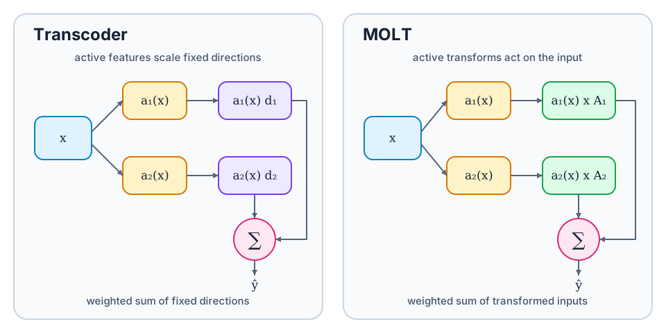
Sparse Mixture of Linear Transforms (MOLT): An interpretable MLP replacement that routes an input through a sparse set of learned low-rank linear maps. Each map has a learned activation condition and an input-dependent output.

The rotation example shows how a transform can describe a geometric operation more compactly than fixed output vectors.

The MOLT Computation

Let the MLP input be a row vector $\mathbf{x} \in \mathbb{R}^{1 \times d}$ . Transform $t$ has a scalar gate

a_t(\mathbf{x}) = \phi(\mathbf{x} \cdot \mathbf{e}_t - b_t),

where $\mathbf{e}_t$ detects the contexts in which the transform should operate, $b_t$ sets its threshold, and $\phi$ is a sparse activation function such as ReLU or JumpReLU. Its contribution to the reconstructed MLP output is

a_t(\mathbf{x})\, \mathbf{x} W_{\text{down},t} W_{\text{up},t},

with $W_{\text{down},t} \in \mathbb{R}^{d \times k_t}$ and $W_{\text{up},t} \in \mathbb{R}^{k_t \times d}$ . The product

A_t = W_{\text{down},t} W_{\text{up},t}

is a $d \times d$ matrix with rank at most $k_t$ . Using these two factors is much cheaper than learning a separate full-rank matrix for every transform. Summing the active contributions gives the MOLT's output:

\hat{\mathbf{y}}_{\text{MLP}} = \sum_t a_t(\mathbf{x})\, \mathbf{x} A_t.

This equation separates when transform $t$ operates, encoded by $a_t$ , from what it does, encoded by $A_t$ . The output direction of $\mathbf{x}A_t$ depends on the input. A single map can therefore relate many input directions to many output directions.

Comparison of a transcoder and a MOLT. The transcoder selects fixed output vectors, while the MOLT selects low-rank maps whose outputs depend on the input vector. — A transcoder latent contributes a scaled fixed decoder vector. A MOLT gate selects a low-rank map, so the contribution changes with the input. Adapted conceptually from Lindsey et al. [3]

Sparse Features and Sparse Transforms

Both methods approximate an MLP with a small number of active units. In a transcoder, each unit contributes along a fixed output direction; in a MOLT, it applies a linear map to the input.

Property	Transcoder	MOLT
Sparse unit	Scalar latent feature	Gated linear transform
Output when active	A scaled fixed decoder direction	A transformed version of the current input
Computational rank per active unit	One output direction	Up to $k_t$ dimensions
Representation and computation	One latent serves as both feature and computational step	Transform represents a computational step only
How it enters a circuit	Usually a feature node	Usually a label or mediator on an edge between features

The inputs that most strongly activate a transcoder feature show when it is used. We can examine its fixed decoder vector to interpret what it contributes to the output. The examples that most strongly activate a MOLT gate reveal when the transform runs. To understand what it does, we also need to inspect how $A_t$ acts on different inputs, because it has no single output direction.

We can use sparse autoencoders to describe the representations before and after a MOLT layer. The proposed workflow learns sparse features in the residual stream at both points, then uses MOLT transforms to explain how source features contribute to target features. Features describe what is represented; transforms help explain how one representation becomes another.

Pause and think: Why is the gate not enough?

Suppose a MOLT gate activates almost exclusively on Spanish text. Have we learned what its transform does?

No. The gate tells us when the map is used. The map could turn a feature for a concept into a feature for a Spanish word, adjust grammatical agreement, pass along punctuation information, or perform several operations depending on the input. We need to inspect how $A_t$ maps particular source directions toward particular target directions.

Training a Sparse Replacement

A MOLT is trained to predict the output of an existing MLP from that MLP's input. A schematic objective is

\mathcal{L} = \left\|\mathbf{y}_{\text{MLP}} - \hat{\mathbf{y}}_{\text{MLP}}\right\|_2^2 + \lambda \sum_t \rho(a_t)\, \|A_t\|_F,

where the first term measures reconstruction error and $\rho$ penalizes transform activity. Weighting activity by the Frobenius norm $\|A_t\|_F$ prevents the model from evading the sparsity cost by shrinking a gate while enlarging its transform matrix [4].

Low-rank maps are cheap to compute and may capture narrowly defined operations, while higher-rank maps can express broader transformations. Preliminary experiments used a mixture of ranks $k_t$ from 32 to 512. With the same total number of parameters, this mixture reconstructed the tested MLP more accurately than giving every transform the same rank [5].

Here, $L_0$ counts the transforms active on an input. Each of those transforms can still affect many coordinates in the residual stream, even when its rank is low. Sparsity refers to how many transforms run, not how many matrix entries are nonzero.

Transform-Mediated Attribution Graphs

Pairing MOLTs with residual-stream feature dictionaries gives each transform a role inside an attribution graph. Let source feature $i$ have activation $z_i$ and decoder direction $\mathbf{d}_i$ , and let target feature $j$ have encoder direction $\mathbf{e}_j$ . Transform $t$ contributes a local source-to-target term proportional to

z_i\, a_t\, \big((\mathbf{d}_i A_t) \cdot \mathbf{e}_j\big).

The source activation and transform gate make the term input-dependent. The inner product measures how strongly the transformed source direction aligns with the target feature's encoder direction. We can label an edge in the attribution graph with the transforms that account for most of its attributed effect. Examples that activate each transform help explain when that connection is used [6].

For the prompt “3 + 5 = 8,” the preliminary analysis traced a connection from a “plus 3” feature to a feature associated with outputting 8. The connection passed through a transform that activated when 5 had recently appeared. In a Spanish vocabulary example, a transform active in Spanish contexts connected a feature associated with “hot” to one associated with producing a word beginning with “cal” [7]. In these graphs, the features are the nodes, and the transforms explain the connections between them.

Raw scores for pairs of features were harder to interpret because large interaction weights can reflect interference rather than meaningful computation. Restricting the graph to the transforms and feature pairs active on a particular prompt makes it easier to interpret what happens on that prompt.

Evidence and Open Questions

On the middle layer of Claude 3.5 Haiku, MOLTs achieved lower mean squared reconstruction error than transcoders with the same parameter count and number of active units. In the scaling comparison, even the smallest MOLT runs offered a better tradeoff between reconstruction error and sparsity than transcoders trained with up to 1,024 times as many floating-point operations [8].

To test mechanistic faithfulness, we can compare how the replacement and the original MLP respond to changes in their inputs. A Jacobian describes how the output responds to small changes in the input. On a separate 18-layer model, MOLT Jacobians were more closely aligned with the MLP's Jacobians than transcoder Jacobians were, at the same number of active units ( $L_0$ ). MOLT Jacobians can have rank much larger than the number of active transforms, whereas a transcoder's local Jacobian rank is bounded by its active feature count [9].

These preliminary experiments measured reconstruction and Jacobian alignment on different models. Individual transforms are still difficult to interpret outside selected attribution graphs. Some appeared to duplicate the role of the features they acted on, while others activated on generic tokens such as “is.” Adding transform labels to the edges also makes the graphs more complicated to inspect than graphs built from transcoders alone [10].

Pause and think: Reconstruction or mechanism?

A MOLT matches an MLP's output with very low error on held-out text. What additional evidence would support the claim that it captured the same mechanism?

Compare how both systems respond to controlled perturbations, including changes large enough to alter which gates or neurons are active. Comparing Jacobians tests their responses to infinitesimally small changes around observed inputs. Larger interventions test whether they still behave alike when the inputs move away from the patterns seen during training.

Mixture of Decoders (MxD) is an independently developed method that also uses a sparse mixture of linear maps. Its transforms can be full-rank because they share parameters through a tensor factorization, while MOLTs use independently learned low-rank factors. On language models with up to three billion parameters, MxD experiments found a better tradeoff between sparsity and reconstruction accuracy than transcoders. The study also evaluated MxD with sparse probing and steering [11].

Learning each low-rank map separately could encourage it to capture a specific geometric operation. Sharing parameters across full-rank maps lets each active map express a wider range of transformations. It remains unclear which design produces transforms that are easier to interpret. The MOLT work examines how transforms connect separately learned residual-stream features, while MxD more directly evaluates how interpretable each active sublayer is as a component of the original dense layer.

Looking Ahead

Crosscoders learn related sets of sparse features across layers or models. Combining these features with conditional transforms could help distinguish a feature that persists unchanged from one that is repeatedly rewritten.

Circuit Tracing and Attribution Graphs explains how these graphs are built and tested. Extending them to MOLTs means tracing which transforms connect each pair of features, keeping the graph readable, and testing those connections through interventions while retaining the MOLT's reconstruction accuracy.