The Scalability Problem
Activation patching is the foundation of causal interpretability: replace an activation, measure the effect, and establish which components matter. But it has a fundamental scaling problem. Each component tested requires a separate forward pass through the model. In GPT-2 Small, testing all 144 attention heads and 12 MLP layers means 156 forward passes. In GPT-3, with roughly 4.7 million neurons, individually testing every neuron is computationally infeasible.
The cost creates a methodological bottleneck: screen only a tractable subset and risk missing structure, or spend enough compute to patch every candidate. A first-order approximation makes a model-wide sweep possible with a small number of passes.
Attribution patching estimates many patching effects from gradients [1]Attribution Patching: Activation Patching At Industrial Scale Using Differential Calculus
Nanda, N.
Blog post, 2023. Path patching asks which connections carry an effect between components [2]Towards Automated Circuit Discovery for Mechanistic Interpretability
Conmy, A., Mavor-Parker, A. N., Lynch, A., et al.
NeurIPS, 2023. Both trade exactness or simplicity for scale and resolution.
Attribution Patching: The Gradient Approximation
Attribution patching approximates the effect of patching every component without performing each patch. A first-order Taylor approximation combines how sensitive the metric is to an activation (the gradient) with how much that activation differs between clean and corrupted runs (the activation difference). Their product estimates the patching effect.Attribution patching is closely related to 'gradient times input' attribution methods from the broader interpretability literature. Instead of multiplying the gradient by the input itself, it uses the difference between clean and corrupted activations, focusing the attribution on task-relevant changes rather than absolute activation magnitudes.
Formally, the estimated patching effect for activation is:
The gradient captures the local sensitivity of the metric to perturbations at . The difference captures how much the activation actually changes between the two runs. Their dot product estimates how much the metric would change if we replaced the corrupted activation with the clean one at that location.
The efficiency gain is dramatic. Full activation patching requires forward passes, where is the number of components. Attribution patching requires exactly two forward passes (one clean, one corrupted) plus one backward pass (to compute gradients). That is three passes total, regardless of model size. For GPT-3 with 4.7 million neurons, this means 3 passes instead of 4.7 million.
When the Approximation Holds
The accuracy of attribution patching depends on whether the first-order (linear) approximation captures the true relationship between activation changes and metric changes.
Where it works well. Transformers are, as Nanda puts it, "shockingly linear objects" [3]Attribution Patching: Activation Patching At Industrial Scale Using Differential Calculus
Nanda, N.
Blog post, 2023. For small activations like individual attention head outputs and individual neurons, the linear approximation is often surprisingly accurate. The patching effect at this scale is genuinely close to linear in the activation perturbation, so the gradient captures most of what matters. Attribution patching at the head level and neuron level typically agrees well with full activation patching on the same components.
Where it breaks down. For large activations such as entire residual streams at a layer, the approximation degrades. Nonlinearities from softmax, MLP activation functions, and LayerNorm all violate the linearity assumption. These nonlinearities mean that the effect of patching an entire layer's residual stream is not well-approximated by a gradient. The Taylor expansion assumes small perturbations, and patching an entire residual stream is a large perturbation.One way to understand this: the gradient gives you the slope of the function at a point. For a linear function, the slope is constant, so the prediction is exact regardless of perturbation size. For a nonlinear function, the slope changes as you move away from the evaluation point, and the prediction becomes increasingly inaccurate for larger perturbations.
The practical implication. Attribution patching is best used as a fast screening tool, not as a substitute for actual activation patching. The recommended workflow is: sweep the entire model with attribution patching to identify the most promising components in a single pass, then verify the top candidates with full activation patching. Think of it as a microscope's low-magnification mode, scan the whole slide quickly, then switch to high magnification on the interesting regions.
Pause and think: When would attribution patching be misleading?
Consider a component whose patching effect is highly nonlinear, for instance, a component where small perturbations have no effect but large perturbations cause a phase transition in model behavior. What would attribution patching report for this component, and how would it compare to full activation patching?
Attribution patching would report a small effect because the gradient at the evaluation point is near zero, while full activation patching would reveal a large finite-change effect. A substantial disagreement is therefore evidence that the local linear approximation is inadequate at that location.
Path Patching: From Components to Connections
Standard activation patching replaces a component's entire output, combining every downstream use of that write. Head might supply task-relevant information to head while also affecting head through an irrelevant route. A whole-output patch measures their net effect but does not identify which downstream consumer uses the information.
Path patching asks a more targeted question: is the specific connection from to important? Instead of replacing 's entire output in the residual stream, path patching replaces only the component of 's output that flows into a specific downstream consumer .Implementing path patching is more involved than standard activation patching. You need to identify how a downstream head reads from the residual stream (through its QKV projections) and selectively patch only the contribution from the upstream head. In practice, this is done by patching the input to the downstream head's query, key, or value computation rather than the upstream head's output directly.
The conceptual shift is from nodes to edges in the computational graph:
- Activation patching tests nodes: "Is component important?"
- Path patching tests edges: "Is the connection important?"
In the IOI circuit, activation patching implicates both S-Inhibition and Name Mover heads [4]Interpretability in the Wild: a Circuit for Indirect Object Identification in GPT-2 Small
Wang, K., Variengien, A., Conmy, A., et al.
arXiv, 2022. Path patching narrows the hypothesis to the route into Name Mover queries, supporting an account in which S-Inhibition changes where Name Movers attend rather than what their value pathway copies.
Automated Circuit Discovery
Path patching, applied systematically, becomes a tool for automated circuit discovery. Conmy et al. developed the ACDC algorithm (Automatic Circuit DisCovery) to do exactly this [5]Towards Automated Circuit Discovery for Mechanistic Interpretability
Conmy, A., Mavor-Parker, A. N., Lynch, A., et al.
NeurIPS, 2023.
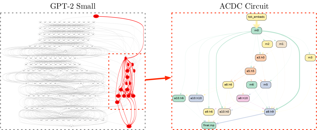
Conmy, A., Mavor-Parker, A. N., Lynch, A., et al.
NeurIPS, 2023
ACDC starts with a chosen computational graph and treats its edges as candidate connections. It then tests edges in an order and prunes those whose removal falls below a selected effect threshold. What remains is a sparse circuit candidate. Because effects can interact, the greedy result need not be globally minimal and can depend on the graph, metric, baseline, ordering, and threshold.
The algorithm proceeds in topological order, working backward from the output:
- Start with all edges in the computational graph
- For each edge (in reverse topological order), temporarily remove it
- If the model's behavior on the task is unchanged, permanently prune the edge
- If behavior degrades, keep the edge
- The surviving edges define the circuit
The threshold for "unchanged" is a tunable parameter, creating a tradeoff between faithfulness (keeping all edges that matter) and minimality (removing as many as possible). A strict threshold keeps more edges and produces a more faithful but less interpretable circuit. A loose threshold prunes aggressively and produces a more minimal but potentially less faithful circuit.
ACDC was validated on the IOI task, where it recovered a circuit closely matching the one Wang et al. found through manual analysis [7]Interpretability in the Wild: a Circuit for Indirect Object Identification in GPT-2 Small
Wang, K., Variengien, A., Conmy, A., et al.
arXiv, 2022. The key advantage is speed: ACDC can screen thousands of edges in hours, while manual circuit discovery took months.
Pause and think: Choosing the pruning threshold
ACDC prunes an edge if removing it changes the model's behavior by less than a threshold . What happens if is set too high? What happens if it is set too low?
If is too high, edges that contribute modestly to the task are pruned, and the resulting circuit may miss secondary components like Backup Name Movers. The circuit becomes more minimal but less faithful. If is too low, the circuit retains many irrelevant edges and provides little simplification over the full model. The goal is to find the threshold where the circuit captures the primary mechanism without excessive noise. In practice, researchers often sweep across multiple threshold values and compare the resulting circuits.
Combining the Tools
Attribution, activation, and path patching answer related questions at different costs. One useful workflow applies them in stages:This sequence is a practical heuristic, not a required recipe. The right validation depends on the model, task, intervention size, and claim being made.
-
Attribution patching for broad screening. Sweep the entire model to identify which components show the largest estimated patching effects. This narrows the search from thousands of components to a manageable set of candidates.
-
Activation patching for confirmation. Run full patching on the top candidates to verify that the gradient approximation was accurate. This catches components where the linear approximation was misleading.
-
Path patching for mechanistic understanding. Once the key components are identified, trace the connections between them. This reveals not just which components participate in the circuit but how information flows between them.
Attribution patching may localize an effect to layer 9; activation patching can test head 9.9 directly; path patching can then ask whether that head receives S-Inhibition information through its queries and copies a name through its OV circuit. Each intervention narrows the causal claim.
To see this full toolkit applied to the most ambitious circuit analysis ever attempted, continue to The IOI Circuit: Discovery and Mechanism.