Activation Patching: Causal Interventions

From Observation to Causation

Mechanistic interpretability begins with observational tools. The logit lens shows what a model would predict if processing stopped at a given layer. Probing classifiers reveal what information is linearly decodable from the residual stream. Attention patterns display where each head directs its focus. These techniques are powerful, but they share a fundamental limitation: they show what information exists in a model's internals, not what information the model actually uses.

A probing classifier might detect part-of-speech information at 95% accuracy from layer 6 activations, yet removing that information might leave downstream performance unchanged. The information was present, but the model did not rely on it. Observation establishes accessibility; testing use requires an intervention.

Activation patching replaces a specific activation in one model run with the corresponding activation from another, then measures the change in behavior [1]. A change supports a causal claim about this intervention and input pair. Interpreting that claim still requires care about what was patched, which baseline supplied the replacement, and how downstream components responded.

The Clean/Corrupted Framework

The basic setup requires two model runs:

A clean run where the model processes a prompt that produces the desired behavior.
A corrupted run where the model processes a modified prompt that produces different behavior.

We then replace specific activations from one run into the other and observe how the output changes.

Consider a concrete example from the Indirect Object Identification (IOI) task:

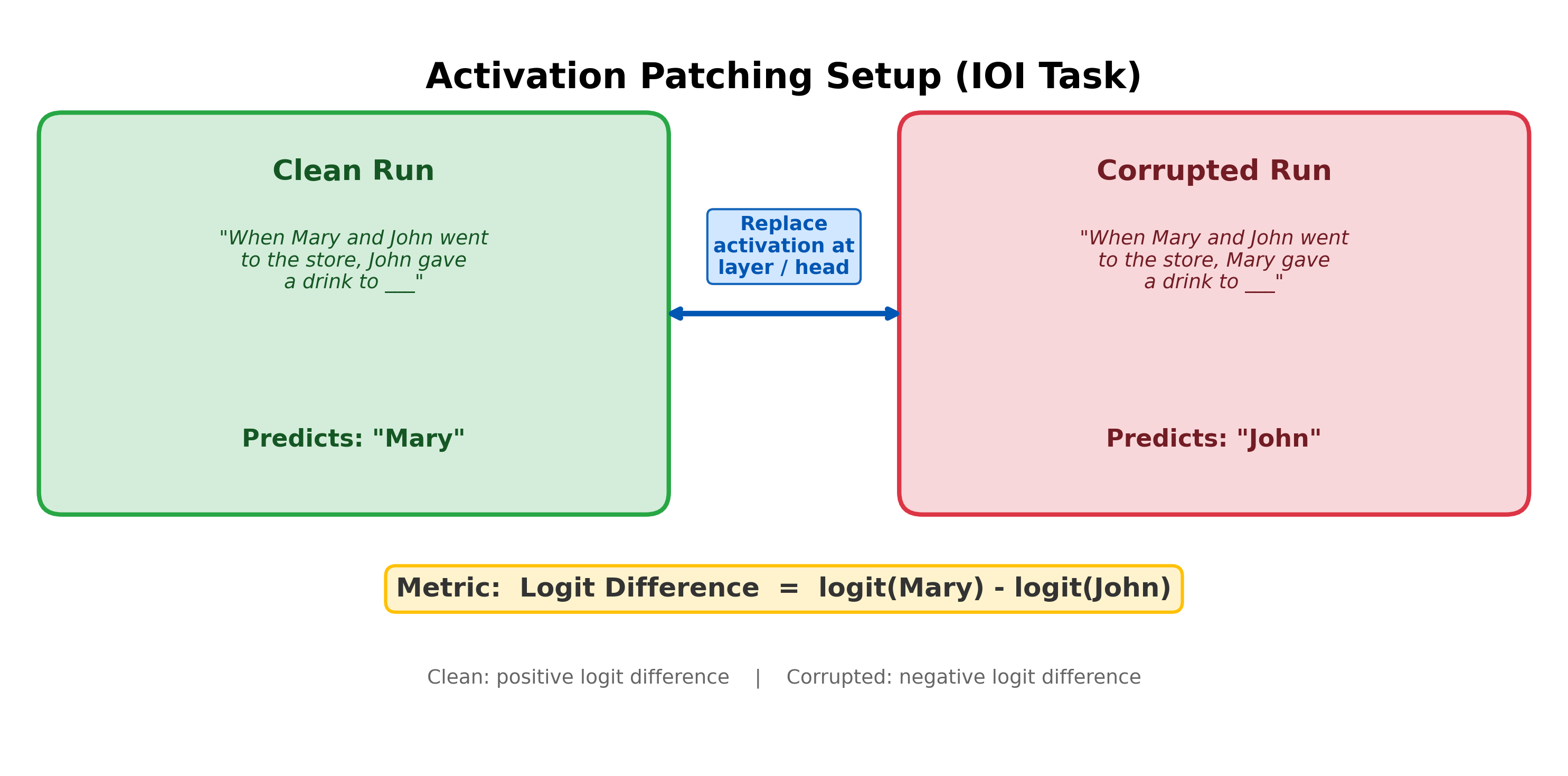
Clean: “When Mary and John went to the store, John gave a drink to ___.” The model predicts Mary, the indirect object.
Corrupted: “When Mary and John went to the store, Mary gave a drink to ___.” The model predicts John, now the indirect object.

Now run the corrupted prompt, but replace one layer or attention head activation with its clean value. If the output shifts back toward “Mary,” that activation mediates some of the difference between the two runs. If it does not, several explanations remain possible: the component may be irrelevant, redundant, poorly matched to the patch, or masked by downstream compensation. Repeating the intervention across locations produces a map of candidate causal sites rather than a finished mechanism.

Activation Patching: Activation patching replaces activation $a_i$ in one run with the corresponding value $a_i'$ from another: $\hat{y} = M(x;\; a_i \leftarrow a_i')$ . The model then recomputes all downstream activations. The change $\hat{y} - y_{\text{original}}$ measures the effect of that particular replacement for this input pair.

Diagram showing the activation patching setup with clean and corrupted model runs side by side, with an arrow indicating activation replacement at a specific layer. — Figure 1: The activation patching setup. Run the model on both clean and corrupted inputs, then replace specific activations from one run into the other to measure causal effects.

What makes a good clean/corrupted pair? The two prompts should differ in exactly one semantically meaningful way:

Good: Swap which name is the subject. This changes who the indirect object is with minimal other changes.
Bad: Use a completely different sentence. Too many confounds make it impossible to tell which difference caused the change.
Risky default: Add large random noise to embeddings. The resulting vectors may be far from those produced by natural tokens, so the experiment can mix the intended corruption with a response to distribution shift.

The cleaner the contrast, the more interpretable the results.

Choosing a metric. How do we measure the effect of patching? The preferred metric is the logit difference:

\Delta L = \text{logit}(\text{Mary}) - \text{logit}(\text{John})

The logit difference is continuous, linear in residual stream contributions, and easy to interpret. Alternatives like probability (nonlinear via softmax, creating artificial sharpness) and accuracy (discrete, hiding gradual effects) are less reliable. Heimersheim and Nanda strongly recommend logit difference, with multiple metrics used to check robustness [2].Activation patching was developed independently by several groups under different names. Vig et al. (2020) introduced 'causal mediation analysis' by applying Pearl's framework to neural NLP. Geiger et al. (2021) formalized 'interchange intervention' within a causal abstraction framework. Meng et al. (2022) used 'causal tracing' with Gaussian noise corruption to trace factual associations. Heimersheim and Nanda (2024) synthesized these approaches into the practical framework now used by the MI community.

Noising vs. Denoising

The direction of the replacement changes the causal question.

Denoising (clean into corrupted): Run the corrupted prompt and replace one activation with its clean value. This asks whether that replacement can restore some of the clean behavior. It resembles a sufficiency test, but the patched component is not acting alone: the rest of the corrupted model still supplies context and downstream computation.Denoising and noising are often described as sufficiency and necessity tests. The analogy is useful if kept local to the intervention. A single patch does not establish philosophical or model-wide sufficiency or necessity, because components interact and the replacement may itself be off-distribution in its new context.

Noising (corrupted into clean): Run the clean prompt and replace one activation with its corrupted value. This asks whether that replacement damages the clean behavior. It resembles a necessity test, but a small effect does not prove the component is dispensable: redundant paths or self-repair may hide its contribution.

These two directions answer different causal questions, and the difference is not merely academic. Sufficiency and necessity are not the same thing. A component can be sufficient without being necessary (if there are backups), or necessary without being sufficient (if it needs help from other components).

The AND/OR gate analogy. Heimersheim and Nanda offer a clarifying analogy [3]:

Serial circuit (AND gate): A then B then C. Every component is necessary. Noising any one breaks the circuit.
Parallel circuit (OR gate): A or B or C. No single component is necessary because the others compensate, but each is sufficient alone.

Noising finds AND-circuit components (serial dependencies). Denoising finds OR-circuit components (parallel/redundant paths).

The IOI circuit in GPT-2 has backup Name Mover heads that become more important when primary Name Movers are disabled. Noising can therefore understate the primary heads' roles, while denoising may still show that restoring their clean activations rescues the corrupted run.

A component can look unimportant in one direction and important in the other. Reporting the patch direction is therefore part of reporting the result, not an implementation detail.

Pause and think: Redundant components

Consider a circuit with two redundant components A and B that each independently produce the correct output. What does noising A show? What does denoising A show? Which gives you more useful information about the circuit's structure?

Noising A would show little or no effect, because B compensates. Denoising A would show a large effect, revealing that A alone carries enough information. In circuits with redundancy, denoising is more informative for identifying individual components.

Ablation: Choosing a Baseline

Activation patching substitutes an activation from one specific run into another. But sometimes we want to ask a simpler question: "What happens if this component contributes nothing?" This is ablation: replacing a component's activation with some baseline value to test whether the model needs it.

Ablation: Replacing a model component's activation with a fixed baseline value (rather than a value from a specific alternative run) to test whether the component is necessary for a behavior. Ablation tests necessity: if performance degrades, the component matters.

The choice of baseline is not obvious, and it affects results in practice.

Zero ablation sets the component's output to the zero vector. This is the simplest option: it removes the component's additive contribution to the residual stream entirely. But zero is often far from the model's natural activation distribution. Downstream components receive an input they would never see during normal operation, so the observed effect may partly reflect the model's response to an out-of-distribution input rather than the component's genuine contribution.

A two-input network for $\max(x,y)$ shows why zero has no universal meaning. For positive inputs, the network can compute

\max(x,y) = \operatorname{ReLU}(x-y) + y.

The hidden value $\operatorname{ReLU}(x-y)=0$ is informative: it says that $y \geq x$ , so the second input is the maximum. Forcing that hidden value to zero does not install an abstract state called “no information.” It makes the network behave as though one branch condition held, whether or not it did. An additive component output can often be removed cleanly with zero, but activations inside nonlinear computations require a causal interpretation of what zero represents at that site.

Mean ablation replaces the activation with its mean over a dataset of inputs. The intuition: the mean activation represents the component's "average" contribution. Replacing with the mean removes the component's input-specific signal while preserving its average effect on the residual stream. This keeps downstream activations closer to their natural distribution than zero ablation does.In practice, mean ablation and zero ablation often agree on which components are important, but they can disagree on magnitude. Components whose mean activation is far from zero, common for MLP layers, which often have a large constant bias term, show substantially different ablation effects under the two methods.

Resampling ablation replaces the activation with a value from a different input. The replacement itself comes from the component's empirical distribution, but pairing it with the current context can still break correlations between components. Multiple resamples are usually needed for a stable estimate. The causal scrubbing framework uses structured resampling to test which distinctions a circuit hypothesis says should be irrelevant.

Optimal ablation replaces the component with one input-independent constant chosen to minimize expected model loss under the ablation [4]:

\mathbf{a}^* = \arg\min_{\mathbf{a}} \mathbb{E}_{X}\!\left[L\!\left(M_{A\leftarrow\mathbf{a}}(X), M(X)\right)\right].

Because the same $\mathbf{a}^*$ is used for every input, it cannot transmit input-specific information through the ablated component. Unlike mean ablation, it accounts for nonlinear downstream computation and the chosen loss. The optimization can still activate substitute behavior or understate a component's role in the intact model, so “optimal” means least disruptive under this objective, not causally neutral.

Mean ablation is cheap and commonly used, but no baseline is neutral. Zero removes an additive update, the mean removes input-specific variation, resampling substitutes another input's variation, and optimal ablation learns the least disruptive constant for a specified loss. Results should be interpreted, and ideally checked, under the baseline that matches the causal question.

Corruption Methods Matter

The choice of how to construct the corrupted input is at least as consequential as the choice of ablation baseline. Zhang and Nanda [5] demonstrated that different corruption methods applied to the same model on the same task can lead to substantially different conclusions about which components matter.

Symmetric Token Replacement (STR) constructs corrupted prompts by swapping key tokens with semantically matched alternatives: "The Eiffel Tower is in [Paris]" becomes "The Colosseum is in [Rome]." Both prompts are perfectly valid sentences the model would encounter naturally, so internal mechanisms operate normally on both. The corruption changes only which factual information the model needs to recall.

Gaussian noise (GN), used by Meng et al. in their ROME causal tracing work, adds noise drawn from $\mathcal{N}(0, 3\sigma)$ to token embeddings. This is simpler to implement (no need to construct paired prompts), but the resulting embeddings are far outside the training distribution.

For factual recall in GPT-2 XL, Gaussian-noise corruption produces a salient peak of MLP importance around layer 16, part of the “early site / late site” pattern reported in the ROME work. Symmetric token replacement produces no comparable peak on the same model and task, and the Gaussian-noise peak was two to five times larger across several configurations. The localization result therefore depends materially on the corruption method.

Why does GN produce inflated results? Zhang and Nanda traced the problem to out-of-distribution activation propagation. Under GN corruption, attention patterns in downstream heads break: Name Mover heads that normally attend to the indirect object with 0.58 probability split their attention diffusely. When upstream components are patched (restored) in a GN-corrupted run, they cannot fix the downstream damage because intermediate components have already been pushed into abnormal operating regimes. Under STR, patching upstream components cleanly restores downstream behavior because all components are operating in-distribution throughout.This finding has practical implications for the ROME literature. The strong localization of factual knowledge to specific MLP layers, which motivated ROME's design choice to edit only mid-layer MLPs, may be partly a consequence of Gaussian noise corruption rather than a faithful reflection of how the model processes facts. This does not invalidate ROME as an editing technique, but it does complicate the interpretability claims that motivated it.

Metric choice matters too. Probability as a metric cannot detect negative components (heads that actively hurt performance), because it is bounded below by zero. When the corrupted-run probability of the correct token is already near zero, components that make things worse cannot reduce it further. Logit difference has no such floor. Zhang and Nanda found that probability and logit difference identify different sets of important heads on the IOI task, with probability missing all three Name Mover heads under some configurations.

When a natural matched pair exists, symmetric token replacement is usually easier to interpret than large embedding noise. Logit difference also avoids the probability floor when the question concerns competition between two answers. Neither choice is universal: the corruption and metric should match the causal question, and robustness checks should report how conclusions change under plausible alternatives.

A Worked Example: IOI in GPT-2 Small

Let us walk through activation patching on the Indirect Object Identification task in GPT-2 Small. This worked example demonstrates the full patching workflow and reveals the sparse circuit structure that makes mechanistic interpretability possible.

Step 1: Establish the baseline. On the clean prompt, the model correctly predicts "Mary" with a positive logit difference:

\Delta L = \text{logit}(\text{Mary}) - \text{logit}(\text{John}) > 0

On the corrupted prompt (where the subject names are swapped), the model predicts "John" with a negative logit difference:

\Delta L = \text{logit}(\text{Mary}) - \text{logit}(\text{John}) < 0

The gap between these two values is what we want to explain: which internal components drive this behavioral difference?

Step 2: Patch layer by layer. For each layer $\ell$ , we replace the corrupted residual stream with the clean one (denoising direction) and measure how much of the logit difference is recovered.

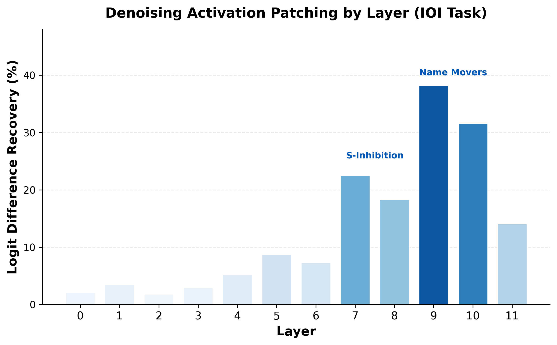
Bar chart showing patching recovery by layer. Layers 0-4 show small effect, layers 5-6 moderate, layers 7-8 large (S-Inhibition heads), layers 9-10 the largest (Name Mover heads). — Figure 2: Layer-by-layer activation patching results on the IOI task. Layers 7-10 carry the most causally important information.

The patching heatmaps localize the behavior at progressively finer resolution:

Layers 0-4: Small effect. Early processing (token embeddings, positional information) does not contribute much on its own.
Layers 5-6: Moderate effect. Induction-style heads begin to contribute.
Layers 7-8: Large effect. This is where the S-Inhibition heads operate, suppressing attention to the duplicated name.
Layers 9-10: The largest effect. The Name Mover heads directly copy the indirect object name to the output logits.

Step 3: Patch individual attention heads. The layer-level results show where in the model the critical computation happens, but not which specific components are responsible. For each of the 144 attention heads (12 layers times 12 heads), we patch the corrupted head output with the clean one and measure recovery.

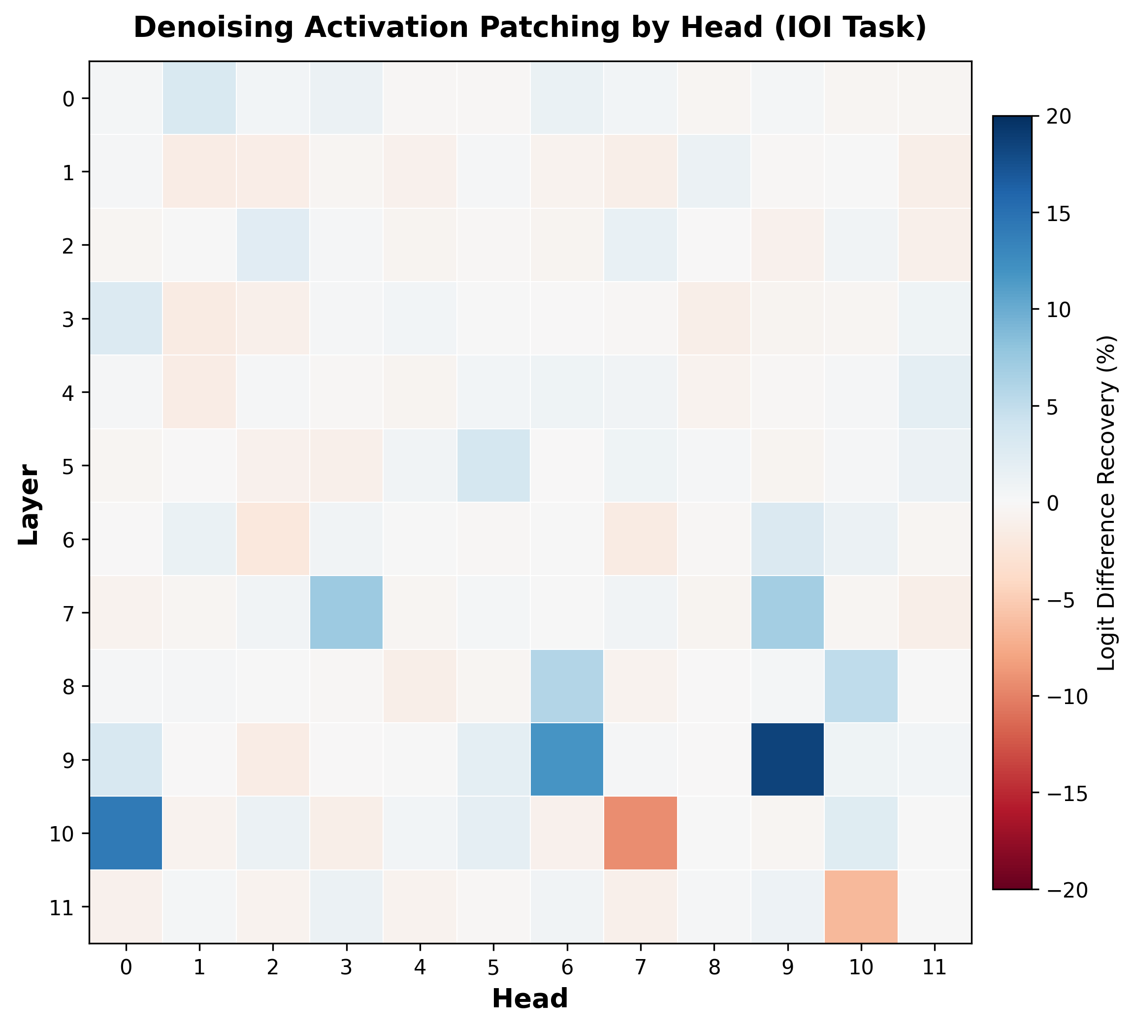
Heatmap showing patching effect for each of 144 attention heads (12 layers x 12 heads). Most cells are near zero. Blue cells at heads 9.9, 10.0, 9.6 show positive effect (Name Movers). Red cells at 10.7, 11.10 show negative effect (Negative Name Movers). — Figure 3: Head-level activation patching results. The IOI circuit involves roughly 10-15 heads out of 144, revealing a sparse structure.

Under this prompt distribution, metric, and patching setup, most heads have near-zero measured effect while a small group stands out:

Blue cells (positive effect): These are the key players. Heads 9.9, 10.0, and 9.6 are the Name Mover heads, each recovering a large fraction of the logit difference. Heads 7.3, 7.9, 8.6, and 8.10 are the S-Inhibition heads, which suppress the wrong answer.

Red cells (negative effect): Heads 10.7 and 11.10 are Negative Name Movers that write against the correct answer on these examples. Their direct effect suppresses the correct-name logit, even though the intact network still solves the task.

Interpretation. Roughly 10 to 15 heads recover much of the measured clean-corrupted difference in this screen. Patching narrows the search from 144 heads to a tractable candidate set. Researchers still need weight analysis, attention patterns, path-level interventions, and tests across prompts to turn those candidates into a circuit account.

For the full analysis of how these heads work together to implement an algorithm for identifying the indirect object, see Wang et al. [6].

A note on interpreting recovery percentages. When we say “patching head 9.9 recovers 38% of the logit difference,” replacing that corrupted activation with its clean value restores 38% of the clean-corrupted gap. This does not mean head 9.9 is “38% of the circuit.” Components can have overlapping or interacting effects, so their recoveries need not add to 100%. The percentage describes one intervention, not a unique partition of causal credit.

Pause and think: Designing a patching experiment

You have a model that correctly identifies sentiment in movie reviews. You want to know whether the model relies on specific adjectives or on overall sentence structure. How would you design an activation patching experiment to test this? What would your clean and corrupted prompts look like?

A good approach: use clean prompts with clear sentiment ("This movie was absolutely brilliant") and corrupted prompts where the adjectives are replaced with neutral or opposite ones while preserving sentence structure ("This movie was absolutely terrible"). If patching the early layers (where token identity is processed) recovers the sentiment, the model relies on the specific words. If patching later layers matters more, the model may depend on higher-level structural features.

Specificity: What Did the Patch Leave Alone?

A patch that changes the target output can also move variables that the interpretation claims are separate. If a residual-stream vector after “Paris” encodes country, continent, language, and token identity, replacing the full vector may change all of them. A large target effect establishes Cause, but an attribute-specific claim also needs Isolate: the same intervention should preserve outputs controlled by neighboring attributes [7].

RAVEL operationalizes the pair with entity attributes. To test a proposed continent feature, patch its value from a Tokyo source into “Paris is in the continent of”; a successful Cause intervention changes the answer to Asia. Then apply the same patch to “People in Paris speak”; a successful Isolate intervention leaves French unchanged. High Cause with low Isolate means the feature is causally effective but entangled.

Specificity controls should match the proposed interpretation. A sentiment patch can be tested on topic and writing style, a factual-recall patch on related attributes, and a refusal intervention on unrelated capabilities. Passing a broad benchmark is useful but weaker than testing the variables most likely to share the patched representation. Choosing Causal Mediators develops selectivity together with faithfulness, sparsity, and generality.

Multi-Source Composition

A single-source patch can transplant the answer rather than the variable used to compute it. Multi-source composition patches proposed variables from different runs into one base computation. The strongest construction uses sources that do not contain the final answer token.

Suppose a hypothesis says one site represents an entity and another represents which attribute to retrieve. Take the entity representation from a prompt that mentions the entity without stating the requested attribute, and take the attribute representation from a second prompt about a different entity. If patching both makes the base run produce the correct value for the new entity–attribute combination, the result cannot be explained by copying the answer from either source. It supports a compositional account in which the two sites mediate separable variables.

The control is stronger than stacking two arbitrary patches. Each source must distinguish the intended variable from plausible alternatives, and single-patch conditions should show what each intervention does alone. A composed output can still depend on unpatched context and downstream model knowledge; it demonstrates that the patched variables combine causally, not that they form a complete mechanism.

Attribution Patching

Full activation patching requires a separate forward pass for every component you want to test. In GPT-2 Small with 144 attention heads and 12 MLP layers, that means 156 forward passes. In GPT-3, with roughly 4.7 million neurons, testing each one individually is impractical. The problem is even worse at the neuron level: individual neurons are often polysemantic, responding to multiple unrelated features due to superposition, so head-level patching may miss important structure. Can we approximate patching without running all those forward passes?

Attribution patching [8] uses a first-order Taylor approximation to estimate what full patching would find. The gradient of the metric with respect to each activation tells us how sensitive the output is to changes at that location. The difference between the clean and corrupted activations tells us how much each activation actually changes. Their product approximates the full patching effect:

\text{Patch effect of } a_i \approx \nabla_{a_i}\mathcal{L} \cdot (a_i^{\text{clean}} - a_i^{\text{corrupt}})

The efficiency gain is enormous. Full activation patching requires $O(n)$ forward passes, one per component. Attribution patching requires only two forward passes plus one backward pass for all components simultaneously. For GPT-3 with 4.7 million neurons, that is 3 passes instead of 4.7 million.

When does this approximation work? Transformers are, as Nanda puts it, "shockingly linear objects." The linear approximation often holds well for small activations like individual head outputs and neurons, where the relationship between activation changes and metric changes is approximately linear.

When does it break? For large activations such as entire residual streams at a layer, nonlinearities from softmax, MLP activations, and LayerNorm invalidate the linear regime. The Taylor approximation assumes small perturbations, and patching an entire layer's residual stream is anything but small.

Best practice: Use attribution patching as a fast screening tool. Sweep the entire model in a single pass to identify the most promising components, then verify the top candidates with actual activation patching. Think of it as a microscope's low-magnification mode, scan the whole slide quickly to find the interesting regions, then switch to high magnification for precise measurement.

For a deeper treatment of attribution patching, including its relationship to path patching and how both are applied at scale, see Attribution Patching and Path Patching.

Path Patching

Standard activation patching replaces a component's entire output. But a head's output flows to many downstream components through the residual stream. Head $H$ might send critical information to head $K$ but irrelevant information to head $J$ . Standard patching cannot distinguish these pathways.

Path patching asks a more refined question: which specific pathway carries the critical information? Instead of patching head $H$ 's output everywhere, patch only the part of $H$ 's output that flows to a specific downstream component $K$ . This isolates the direct $H \to K$ connection from other paths through the residual stream.

The shift is from nodes to edges in the computational graph. Activation patching tests whether component $H$ is important. Path patching tests whether the specific connection $H \to K$ is important. This finer resolution reveals the wiring of the circuit, not just which components participate.

Path patching was central to the IOI circuit analysis [9], where it revealed how information flows between the head classes: from Duplicate Token heads through S-Inhibition heads to Name Mover heads. Without path patching, we would know which heads matter but not how they communicate.

Conmy et al. extended this idea into the ACDC algorithm (Automatic Circuit DisCovery), which automates path patching to systematically prune edges and discover circuits [10]. ACDC starts with a fully connected computational graph and iteratively removes edges whose patching effect falls below a threshold, leaving behind the minimal circuit.

Confounds: Self-Repair and Compensation

Activation patching directly tests interventions on model internals, but it has a systematic blind spot: self-repair. Later components may compensate for an ablation or patch, making the measured effect smaller than the component's contribution in the unperturbed run.

Several mechanisms contribute to self-repair. LayerNorm rescaling accounts for a significant fraction: when a component's contribution is removed from the residual stream, the magnitude of the stream changes, and LayerNorm renormalizes it. This mechanical rescaling can recover up to 30% of the ablated effect without any "intelligent" compensation [11]. Backup components provide another source: heads that are nearly inactive under normal operation activate when primary components are removed, picking up their function. The IOI circuit's Backup Name Movers are the canonical example. Beyond these identified mechanisms, a substantial fraction of self-repair remains unexplained [12].

The practical consequence is that an ablation effect is not an intrinsic percentage of “importance.” Compensation can make the measured change smaller than a component's role in the intact computation, while an implausible replacement can make it larger. Report the intervention, baseline, and metric, then look explicitly for changes in downstream components.

Resample ablation replaces a component's activation with a value from another input. The replacement is drawn from an empirical marginal distribution, which can be more plausible than zero, but it may be inconsistent with the current context. Mean ablation makes a different compromise. Comparing plausible baselines is more informative than treating one as universally correct.

For a deeper treatment of self-repair as a general phenomenon, including the known mechanisms and open questions, see Self-Repair in Language Models.

The Causal Toolkit

We now have three levels of causal analysis, each suited to a different stage of investigation:

Activation patching tests which components matter by replacing entire activations. It operates at the node level.
Attribution patching provides fast screening of all components through gradient approximation, making it practical to survey even the largest models.
Path patching tests which connections between components matter, operating at the edge level.

Together, these tools can move an investigation from “something changes near layer 9” to a testable claim that a particular head sends task-relevant information along a particular path. The IOI circuit article shows how researchers combined several such tests into a detailed circuit account, and where that account still requires judgment.