Why Attention?
Consider the sentence: "The cat sat on the mat because it was tired." What does "it" refer to? For a human reader the answer is obvious: "it" means the cat. But arriving at this answer requires looking back across the sentence and connecting a pronoun to the noun it references. A model that processes each token in isolation, without any ability to look at other positions, has no way to make this connection.
A simple feed-forward network applied independently at each position treats every token as if the rest of the sequence does not exist. It can transform each token's representation, but it cannot move information between positions. Pronoun resolution, subject-verb agreement, long-range dependencies: none of these are possible without some mechanism for tokens to communicate with one another.
The attention mechanism solves this problem [1]Attention Is All You Need
Vaswani, A., Shazeer, N., Parmar, N., et al.
NeurIPS, 2017. It provides a structured way for each token to look at every other token in the sequence, decide which ones are relevant, and gather information from them. Rather than processing tokens in isolation, attention lets the model build context-dependent representations where each token's output reflects the entire input it has seen so far.
Queries, Keys, and Values
Attention organizes the communication between tokens around three learned roles. Every token simultaneously plays all three:
Attention (Intuition): Each token participates in attention through three projections. The query () asks "what am I looking for?", the key () advertises "what do I contain?", and the value () provides "what information do I send if attended to?"
Each role is produced by multiplying the current residual-stream representation by a learned weight matrix. For a token at position with input , the three projections are:
The projection matrices map the input down to a -dimensional query/key space, while maps to the value space. In the first layer, the input derives directly from token embeddings and positional information. In later layers it also contains contextual updates from earlier attention and MLP blocks. These are three different "views" of the same input, each optimized by gradient descent for a different purpose during training. Activations are row vectors throughout this curriculum and weight matrices act on the right, which matches the tensor shapes in PyTorch and TransformerLens.
The Attention Equation
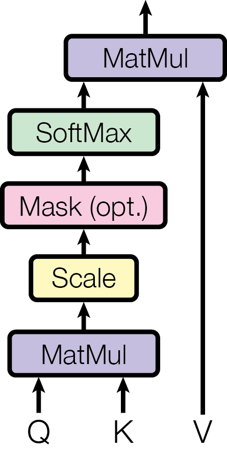
Vaswani, A., Shazeer, N., Parmar, N., et al.
NeurIPS, 2017
With queries, keys, and values defined, the attention mechanism proceeds in three steps: compute relevance scores, normalize them into weights, and use the weights to mix value vectors.
Step 1: Dot-product scores. How much should token attend to token ? The model measures this by computing the dot product between the query of token and the key of token :
A large dot product means the query and key point in similar directions, indicating the model has learned that these two tokens are relevant to each other.
Step 2: Scaling. The raw dot-product scores grow in magnitude with the dimension , which can push the softmax into regions with vanishingly small gradients. The fix is simple: divide by :
Step 3: Softmax normalization. The scaled scores are passed through a softmax to produce a probability distribution over positions:
Now and . Each weight tells us how much attention token pays to token .
The output. The final output for token is a weighted sum of value vectors:
In plain terms: gather information from other tokens, weighted by relevance. Tokens with high attention weight contribute more to the output; tokens with near-zero weight are effectively ignored.
Putting it all together in matrix form, where , , and stack the queries, keys, and values for all tokens:
This equation describes one attention operation [3]Attention Is All You Need
Vaswani, A., Shazeer, N., Parmar, N., et al.
NeurIPS, 2017. A transformer gains depth and computational power by running several such heads in parallel, mixing their outputs with MLPs, and repeating the process across layers.
A Worked Example
To make the attention equation concrete, we trace a single attention head on a 3-token sequence with . The tokens are A, B, and C, and we compute the attention output for token C (the final position).
Setup. Suppose the query, key, and value vectors are:
| Token | Query | Key | Value |
|---|---|---|---|
| A | , | ||
| B | , | ||
| C |
We only need C's query (since we are computing attention from position C) and all three keys and values.
Step 1: Dot-product scores. Token C's query is compared against each key:
Step 2: Scale by . With , we divide by :
Step 3: Softmax. Converting to attention weights:
Token C attends most strongly to itself (50%), with equal attention to A and B (25% each). The self-attention is strongest because C's key aligns most with its own query (dot product of 2 vs. 1).
Step 4: Weighted sum of values. The output for token C is:
The output is dominated by C's own value vector, with smaller contributions from A and B. This is the information that this attention head writes to the residual stream at position C.
The dot products between queries and keys determine the attention pattern: who attends to whom. The values do not affect those weights; they supply the information mixed according to them. Separating the where from the what gives us the QK/OV circuit decomposition developed later.
Self-Attention and Causal Masking
In self-attention, the queries, keys, and values all come from the same input sequence. Given an input matrix (one row per token), we compute , , and . The sequence attends to itself: every token can look at every other token and decide what information to gather. This is how a transformer lets all positions interact in a single step, producing context-dependent representations where each token's output reflects its relationship to the entire input.
For each token position, self-attention performs a complete information-gathering operation: it examines all other positions via the query-key match, decides how much to attend to each via softmax, collects the relevant information as a weighted sum of values, and writes the result back. Each token's output is therefore a context-dependent mixture of all tokens' value vectors.
In decoder-only transformers (such as GPT), there is an additional constraint: each token can only attend to itself and earlier tokens. This is enforced by setting for all before the softmax, which drives those attention weights to zero. This is called causal masking. The reason is simple: during autoregressive generation, future tokens do not exist yet. The model must predict the next token using only the past, so the attention mechanism must respect this constraint during both training and inference.Causal masking gives mechanistic interpretability a clean experimental setup. At each position i, we know exactly what information is available to the model: tokens 0 through i. This makes it possible to reason precisely about what the model could and could not have used to produce its output.
Multi-Head Attention
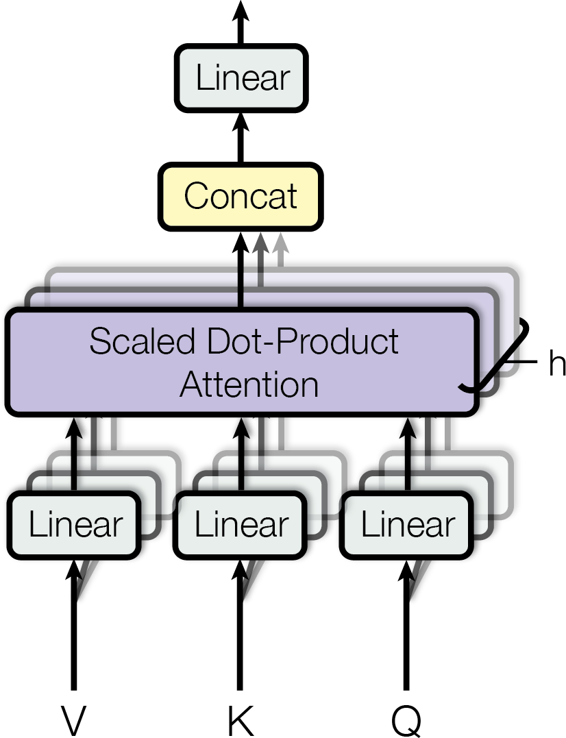
Vaswani, A., Shazeer, N., Parmar, N., et al.
NeurIPS, 2017
A single attention head produces one distribution over source positions for each destination position. Language often benefits from several such distributions at once: one head can favor the previous token, another the sentence's subject, and another an earlier instance of a repeated pattern.
The solution is to run multiple attention heads in parallel, each with its own learned projection matrices. Each head has its own , , and , and computes attention independently:
The outputs of all heads are concatenated and projected through a final output matrix :
Why is needed? Because each head operates in a small -dimensional subspace, its output cannot be added directly to the -dimensional residual stream. The output matrix maps the concatenated head outputs back into the full residual stream space. It also lets each head learn how to write its result back: which dimensions of the residual stream to update and with what mixture. In mechanistic interpretability, the combined matrix (the slice of corresponding to head ) is called the OV circuit of a head: it determines what information the head moves from source to destination.
Parallel Heads: Within one attention layer, each head computes its own QK pattern and OV write from the same input state. Their outputs are then summed into the shared residual stream, where later components can combine them.
In the standard parameterization, , so splitting one full-width attention operation into heads does not increase the leading projection-parameter count. It does give the layer separately parameterized routing patterns and writes, which may specialize differently.Each head's QK and OV matrices are low rank, with rank at most the head dimension. That constrains any one head's routing and writing capacity, although several heads and later layers can combine their effects.
Researchers have identified heads with recurring patterns on defined distributions. Previous-token heads place substantial weight on the preceding position. Induction heads support repeated-pattern completion, and Name Mover heads copy candidate names in the IOI task. These labels summarize tested behavior, not everything a head does on all inputs.
To see why multiple heads matter, consider the sentence "The tired cat sat on the mat because it was tired" at the token position "it." Different heads can extract different relationships from the same position simultaneously:
- Head A might attend from "it" back to "cat," resolving the pronoun to its referent.
- Head B might attend from "it" to the first "tired," tracking which property is being referenced.
- Head C might attend from "it" to "sat," tracking the main verb of the clause.
Separate heads make it easier to represent all three relationships at once. Each head's QK circuit can produce a different relevance pattern, while its OV circuit can move different information. Their combined outputs can therefore carry the referent, its property, and the action from the same attention layer.
An attention head is one information-moving operation, but its behavior may change with the input and may only make sense together with other heads. Mechanistic analysis therefore studies both individual heads and the circuits they form.
Multi-Query Attention
Autoregressive generation exposes a cost that parallel training hides. After processing a prompt, the model generates one new token at a time. Each layer computes a query for the new token and compares it with keys for every earlier token, then mixes the corresponding values. Recomputing all earlier keys and values would waste work, so inference systems store them in a key-value (KV) cache.
In ordinary multi-head attention (MHA), every head has its own key and value projections. A layer with query heads therefore caches key vectors and value vectors per previous token. Long contexts make repeatedly loading this cache a major memory-bandwidth cost.
Multi-Query Attention (MQA): MQA keeps distinct query heads but uses one key projection and one value projection shared by all of them.
For query head , MQA computes
The queries can still ask different questions, producing different attention patterns against the shared keys. Those patterns then mix the same shared value vectors in different proportions. Each head also retains its own slice of the output projection, so the resulting writes to the residual stream can differ.
Shazeer introduced MQA to reduce the memory traffic of incremental decoding [5]Fast Transformer Decoding: One Write-Head is All You Need
Shazeer, N.
arXiv, 2019. Ignoring batch size and bytes per number, a decoder with layers, context length , head width , and key-value heads stores a cache proportional to
The factor 2 accounts for keys and values. Standard MHA has ; MQA has , reducing this part of the cache by a factor of . Queries are not cached for previous tokens because only the current destination token's queries are needed at each decoding step.
The sharing is a capacity tradeoff rather than a free algebraic rewrite. MQA forces all query heads to use the same key features for deciding where to read and the same value features for deciding what source information is available. The original experiments reported much faster decoding with only minor quality degradation in their tested models, but the size of that tradeoff depends on the model and training setup [6]Fast Transformer Decoding: One Write-Head is All You Need
Shazeer, N.
arXiv, 2019.
Grouped-Query Attention
MQA chooses the most aggressive sharing possible. Grouped-query attention (GQA) places intermediate points between one shared key-value head and a separate pair for every query head [7]GQA: Training Generalized Multi-Query Transformer Models from Multi-Head Checkpoints
Ainslie, J., Lee-Thorp, J., de Jong, M., et al.
EMNLP, 2023.
Grouped-Query Attention (GQA): GQA partitions query heads into groups. Every query head keeps its own query and output projections, while all heads in one group share a key projection and a value projection.
Assume divides and number both from zero. Query head uses group
so its output is
The endpoints recover the other architectures. Setting gives MHA, with one key-value pair per query head. Setting gives MQA. Values strictly between them are GQA. Ainslie et al. introduced GQA alongside a method for converting existing MHA checkpoints with additional training; in their experiments, uptrained GQA approached MHA quality with inference speed comparable to MQA [8]GQA: Training Generalized Multi-Query Transformer Models from Multi-Head Checkpoints
Ainslie, J., Lee-Thorp, J., de Jong, M., et al.
EMNLP, 2023.
The visualization fixes eight query heads and varies the number of key-value heads. Lines show which queries share a key-value projection. The cache bar shows the key-value cache relative to eight-head MHA under the simplifying assumption that all heads have the same width.
Scroll the diagram horizontally to see every query head.
| Architecture | Query heads | Key-value heads | Relative KV-cache size |
|---|---|---|---|
| MHA | |||
| GQA | , where | ||
| MQA |
For mechanistic interpretability, “head” now names a partly shared computation. Two query heads in the same GQA group have different query-key (QK) circuits because their query matrices differ, but the key-side read is shared. Their output-value (OV) circuits use the same value matrix and different slices of , so they can select different source positions and write different results despite sharing part of the pathway. Ablating a shared key or value projection intervenes on every query head in its group; ablating one query head's output does not.
Pause and think: What remains head-specific?
An eight-query-head GQA layer has two key-value heads. If query heads 0 through 3 share one key-value group, must they have identical attention patterns and residual-stream writes?
No. They share keys and values, but each has its own query projection, so its query-key scores and softmax pattern can differ. Each also has its own output-projection slice, so differently weighted mixtures of the shared values can be written along different residual directions. Intervening on the shared value projection affects all four heads, while intervening after one head's weighted sum can isolate that head's output.
Pause and think: From architecture to interpretability
If attention heads move information between positions, what determines which information gets moved and where it goes? The query and key matrices determine the "where" (which positions attend to which), while the value and output matrices determine the "what" (which information gets read and written). Decomposing attention into these two circuits, the QK circuit and the OV circuit, is one of the first steps in mechanistic interpretability.
Looking Ahead
Attention moves information between positions. Each transformer layer also contains an MLP, which transforms each position separately. The next article explains the MLP computation and examines evidence for interpreting some neurons as key-value-like memories.
After that, layer normalization addresses the practical complication of keeping activations stable across many layers, and the QK/OV circuit decomposition formalizes the two-circuit structure hinted at above into the mathematical framework that underpins mechanistic interpretability.