Discovering and Interpreting Neural Manifolds

A Curve Is a Hypothesis, Not Yet an Explanation

The previous article showed that concepts can form circles, simplices, and other multi-dimensional structures. It is tempting to run PCA, see a curve, and declare that the model has learned a manifold. That conclusion moves too quickly.

A projection can bend or separate points even when the high-dimensional organization is different. Prompt templates can introduce nuisance variation. A smooth color gradient can appear because the labels were used to choose the projection. Most importantly, a representation can correlate with a variable without being used by the model.

Suppose activations for ages from 10 to 100 trace a loop in a three-dimensional plot. A useful analysis must answer at least four questions:

1. Is the apparent structure low-dimensional in the original activation space?
2. Does it generalize to prompts that were not used to fit it?
3. Do positions along it correspond consistently to age rather than a prompt artifact?
4. Does changing the representation along the structure change the model's computation as predicted?

The object we are trying to establish is therefore stronger than a visualization.

Neural Manifold: A low-dimensional, possibly curved set in activation space on or near which a family of model states lies. The manifold has its own coordinates and geometry even though it is embedded in a much larger activation space.

If a model layer has width $d=4096$, its activations live in an ambient space $\mathbb{R}^{4096}$. A one-dimensional curve inside that space still needs only one local coordinate, such as age or character count, to specify a point on the curve. Its intrinsic dimension is one. A surface parameterized by line width and character count has intrinsic dimension two, regardless of the ambient width.

This distinction is why a manifold is not just another name for a subspace. A $k$-dimensional linear subspace is flat and closed under linear combinations. A $k$-dimensional manifold can curve through many linear dimensions while remaining locally describable by $k$ coordinates.

A Practical Discovery Workflow

Manifold analysis works best when it starts with a concrete variable and a controlled dataset. For a cyclic variable, we might collect activations from matched prompts containing each weekday. For a continuous variable, we might vary an age while holding the rest of the sentence fixed. The activation site, token position, prompt distribution, and target variable should be specified before choosing a flattering projection.

The first pass is exploratory. Center the activations and inspect PCA or another dimensionality reduction method. PCA is especially useful because its explained variance quantifies how much of the cloud lies in a linear subspace. It does not, by itself, estimate the dimension of a curved manifold. A circle has intrinsic dimension one but needs two principal components; a sufficiently twisted one-dimensional curve may need many.

Next, fit a coordinate model. When the intrinsic variable is known, a supervised fit is often the cleanest test. A circle can be parameterized by sine and cosine coordinates. An ordered concept can use a spline through concept centroids. A two-variable family can use a fitted surface. Unsupervised manifold-learning methods are useful when the coordinates are unknown, but they add choices about neighborhood size, metric, and topology that must be tested for stability.

Finally, evaluate on held-out contexts. A credible result should survive new prompt templates, paraphrases, and nuisance variables. Useful checks include:

• reconstruction error from the fitted manifold compared with linear and shuffled-label baselines;
• stability of intrinsic coordinates across layers, datasets, and random seeds;
• local neighborhood preservation, not only the appearance of a global projection;
• decoding the target variable from manifold coordinates on held-out prompts;
• interventions that move, ablate, or patch the proposed coordinates.

Separate Shape, Dimension, and Topology

The manifold's intrinsic dimension asks how many local coordinates vary independently. Its shape describes how distances and curvature behave. Its topology describes global connections that survive smooth deformation: whether the object is an open curve, a loop, a surface with a hole, or several disconnected components.

Ages and weekdays can both have intrinsic dimension one, but an age sequence is an open curve while weekdays form a loop. A coordinate that works for ages has two endpoints. A weekday coordinate must identify the end of Sunday with the beginning of Monday. Fitting both with an unconstrained line would get the dimension right and the topology wrong.

Global projections can also introduce false crossings. A curve that appears to intersect itself in two dimensions may pass through two well-separated regions in the original activation space. Conversely, a method that preserves local neighborhoods can tear a real loop open to display it. The plot is evidence about the output of a visualization algorithm, so topology should be checked with distances and neighborhoods in the original or carefully chosen reduced space.

Many manifolds need more than one coordinate chart. Longitude and latitude work over most of a sphere but become singular at the poles; no single flat map represents the whole surface without distortion. Neural manifold analyses face the same issue when a concept has branches, boundaries, or multiple contexts. A collection of local fits can be more faithful than forcing one global spline through every point.

Baselines That Catch Convenient Stories

A flexible manifold fitter can trace almost any finite point cloud. The relevant question is not whether a curve can be drawn, but whether its inductive assumptions predict new data better than simpler explanations.

Start with a matched linear baseline. Compare a nonlinear fit against PCA using the same training examples and held-out prompts. Then shuffle the concept labels before fitting. If the original and shuffled pipelines perform similarly, the apparent semantic ordering may come from generic activation density or prompt structure. Fit on one template family and test on another to detect template leakage.

Centroids require their own care. Averaging many activations suppresses noise and can reveal a stable concept structure, but it can also create points the model never produces. Report both the geometry of individual activations and the geometry of centroids. A smooth centroid curve surrounded by broad, overlapping clouds supports a weaker claim than tight local neighborhoods ordered along the same curve.

Layer and token selection can become hidden researcher degrees of freedom. If dozens of sites were searched, the best-looking layer is exploratory evidence. A confirmatory test should freeze that choice and evaluate a new dataset. The same principle applies to PCA rank, spline degree, neighborhood size, and distance metric.

Pause and think: One dimension or two?

Points sampled from a circle require two PCA components for accurate linear reconstruction. How many intrinsic dimensions does the circle have?

Only one. A single angle specifies a point locally on the circle. The two PCA components measure the dimension of the smallest flat subspace containing the circle, not the manifold's intrinsic dimension. This is one reason to report both quantities.

From Representation Geometry to Geometric Computation

Finding a stable manifold tells us how a variable is represented. Mechanistic interpretability asks a further question: what computation does the model perform on that representation?

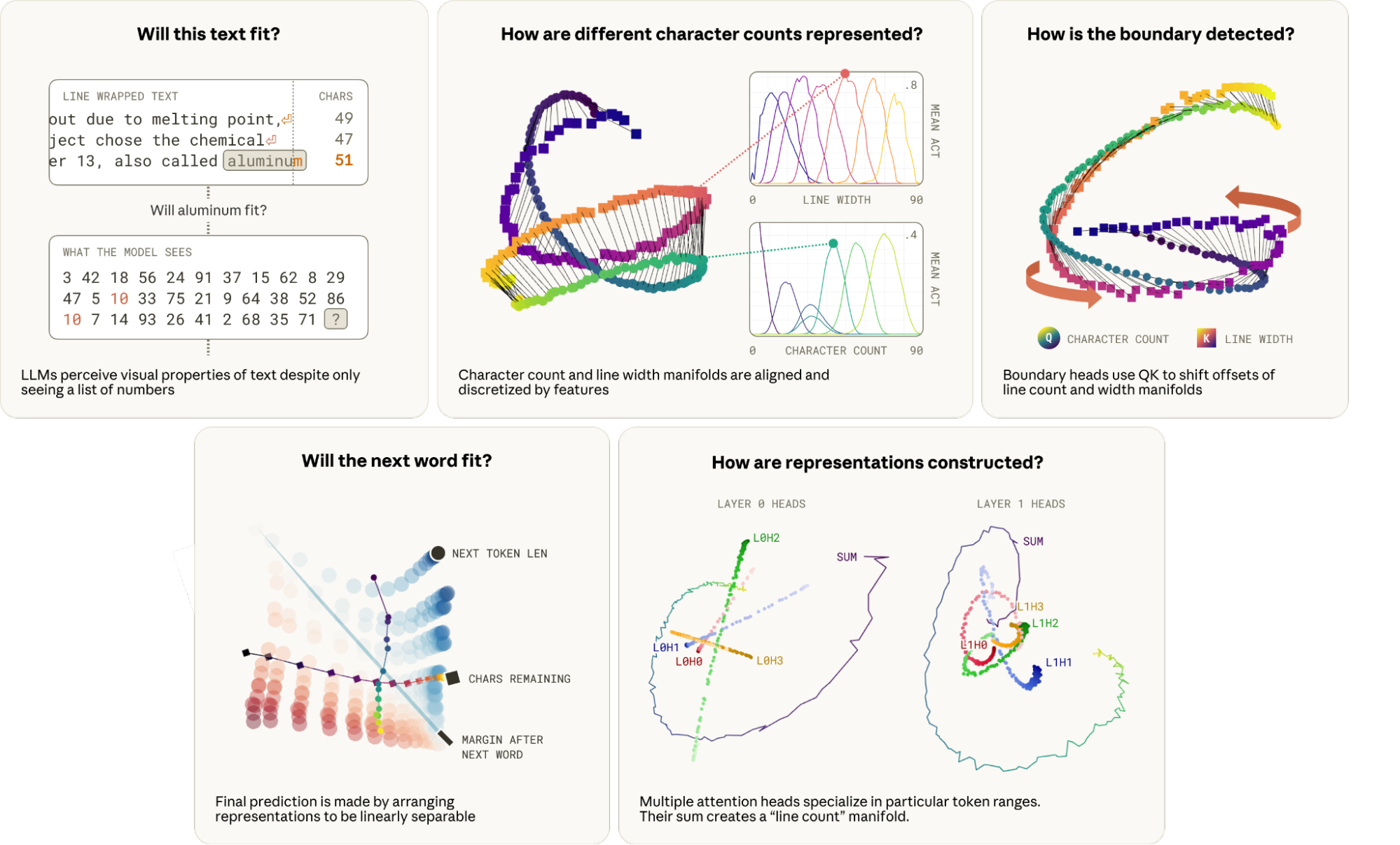
Gurnee et al. studied a language model performing fixed-width line breaking [1]When Models Manipulate Manifolds: The Geometry of a Counting Task
Gurnee, W., Ameisen, E., Kauvar, I., et al.
arXiv, 2026. The model receives text encoded as tokens but must decide whether the next word will cross a character boundary, a task that depends on visual length. Activations encode character count and target line width as curved, low-dimensional structures. Ten crosscoder features provide local coordinates along the character-count curve, while a six-dimensional subspace captures most of its variance.

The attention mechanism does more than read these structures. Query-key interactions transform and align the character-count and line-width manifolds so that compatible values meet. Several heads use slightly different offsets to estimate how many characters remain. Their combined output arranges the relevant states so that the final fit-or-break decision becomes linearly separable.

Subspace ablation showed that removing the count representation damaged line-break predictions. Activation patching changed the model's boundary behavior in the direction predicted by the patched count. Analysis of the attention heads then explained how the two represented quantities were compared. The evidence moves from geometric regularity, through causal dependence, to an account of the transformation.

Geometric Computation: A computation described in terms of transformations, alignments, or comparisons of structured activation sets, rather than only operations on isolated feature directions.

The description is still compatible with ordinary transformer operations. Attention and MLPs remain algebraic functions of vectors. “Geometric computation” names a useful higher-level account of what those operations do to a family of related states.

Three Different Causal Questions

Interventions on a manifold can test several claims, and the intervention should match the claim.

An ablation asks whether the represented family is necessary for a measured behavior. Removing the manifold's ambient subspace can answer this coarsely, but it may erase unrelated variables that share the same dimensions. A local tangent-space ablation is more targeted, although the tangent changes from point to point.

A patch asks whether moving a state from one intrinsic coordinate to another transfers the corresponding variable. Patching a “47 characters” state into a context with 40 characters should shift the boundary prediction in a specific direction. Matched controls should preserve prompt identity and change only the proposed coordinate as closely as possible.

A path intervention asks whether the connections and distances within the structure matter. It compares multiple intermediate states between shared endpoints. Smooth, ordered behavioral changes support the topology and geometry of the proposed representation, not only the causal importance of its span. The next article uses exactly this distinction.

These tests can disagree. A subspace may be necessary even if the fitted curve is wrong. Endpoint patches may work while intermediate paths leave the natural activation distribution. Conversely, a stable geometry may be epiphenomenal if interventions along it do not affect the task. Reporting the separate outcomes prevents “causal manifold” from becoming one oversized claim.

Features and Manifolds Are Two Resolutions of One Object

Feature-based and geometric analyses can look like competing ontologies. One asks which sparse directions are active. The other asks where an activation lies on a continuous structure. The line-breaking result suggests that they can be complementary.

Imagine covering a curved road with short straight paving stones. Each stone is a good local approximation, while the sequence of stones reveals the road's global shape. An SAE dictionary element can play the role of one paving stone: it responds strongly over a local region of the manifold. A group of co-varying elements can then parameterize a structure that no single element captures.

Bhalla et al. formalize the question as whether an SAE compactly captures a concept manifold [3]Do Sparse Autoencoders Capture Concept Manifolds?
Bhalla, U., Fel, T., Rager, C., et al.
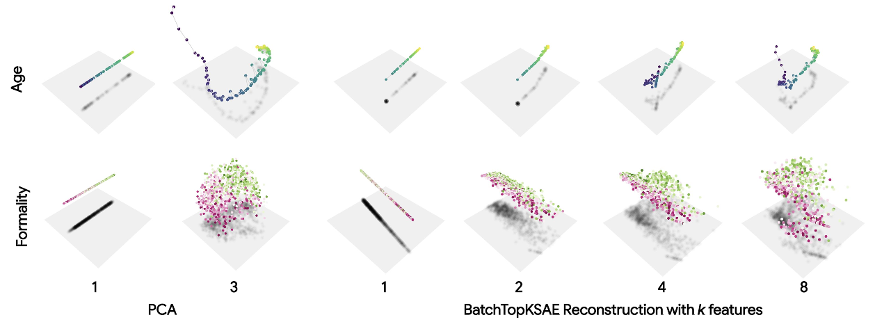
arXiv, 2026. Compact capture means that one small, stable set of decoder features spans the manifold well. The set should not need to grow much beyond the manifold's ambient linear dimension. This is stronger than reconstructing each activation accurately with whichever features happen to fire.

Their experiments distinguish three broad outcomes:

• In compact capture, a small shared group spans the manifold.
• In shattering, different regions depend on nearly disjoint feature groups.
• In dilution, many overlapping and partly redundant features participate, with no small stable group explaining the whole structure.

On synthetic manifolds, compact capture appeared only in a limited sparsity regime. On language-model activations, several SAE variants usually reconstructed manifold regions with localized, overlapping features instead. Adding features improved reconstruction gradually beyond the ambient dimension, a pattern more consistent with dilution than compact capture.

A feature selective for years ending in 7 may not represent the complete concept “year.” It may be one localized detector in a coordinate system distributed across many features. Likewise, several day-selective features need not be redundant mistakes. Their joint activation pattern may trace a circular day-of-week manifold.

A slant-rhyme example makes the failure mode vivid [5]The World Inside Neural Networks
Geiger, A., Lubana, E. S., Fel, T., et al.
Goodfire, 2026. The full activation structure organized words by phonological ending, from close rhymes toward weaker ones. Yet automated descriptions of the individual SAE features focused on local lexical coincidences, such as words beginning with “Hor,” correlation terminology, or absorption-related words. None named the phonological continuum visible at the group level. A feature dashboard could therefore describe every tile while missing the road they collectively pave.

Recovering Structure from Feature Groups

If the manifold is distributed across many sparse features, decoder-vector similarity is not always enough to group them. Nearby local detectors can point in different directions because the manifold curves. Distant detectors can have similar decoder directions by accident. Marginal activation correlation also confounds direct relationships with shared context.

Bhalla et al. instead fit a pairwise maximum-entropy model to SAE activations [6]Do Sparse Autoencoders Capture Concept Manifolds?
Bhalla, U., Fel, T., Rager, C., et al.
arXiv, 2026. Its pairwise couplings measure conditional co-activation: whether two features tend to participate together after accounting for the other modeled features. Clustering that interaction graph recovered groups associated with temperature, color, political orientation, and statistical uncertainty. Within a group, the activation pattern supplies a coordinate system for the underlying concept family.

Moving from isolated features to a manifold hypothesis can follow a six-step workflow:

1. Collect sparse feature activations over a broad, relevant dataset.
2. Build a graph from conditional co-activation or another relation that controls for common causes.
3. Cluster the graph to propose feature groups.
4. Inspect activating examples and visualize each group's joint activations.
5. Fit and validate intrinsic coordinates on held-out data.
6. Test the group with ablation, patching, or coordinated steering.

The graph is a discovery tool, not proof that every cluster is a coherent concept. Dataset frequency, feature splitting, and the SAE training objective all influence the learned interactions. Semantic labels should come after examining the geometry and testing it outside the discovery set.

Pause and think: What would a single-feature test miss?

Suppose seven SAE features fire most strongly on Monday through Sunday, with smooth overlap between neighboring days. Testing each feature separately finds seven narrow causal effects. What additional claim would require testing the group?

The group-level test could establish that their joint state encodes position on one circular variable and that coordinated movement around the circle produces the expected transitions. Individual interventions cannot reveal the topology connecting the seven local detectors.

What Counts as Strong Evidence?

A manifold claim is most convincing when representation, computation, and intervention agree.

Representational evidence shows that a low-dimensional fit generalizes and beats suitable baselines. Computational evidence identifies model components that transform or compare the intrinsic coordinates. Intervention evidence shows that changing those coordinates produces a specific downstream effect while preserving unrelated behavior.

No single diagnostic is decisive. High explained variance can describe an unused correlate. A causal subspace can contain several entangled variables. A successful intervention can leave the data manifold and exploit an unnatural pathway. Even a clean one-dimensional coordinate may be only one of several equivalent parameterizations.

The strongest conclusions are therefore conditional and layered: in these models, layers, prompts, and activation sites, this fitted structure predicts held-out states; these components transform it in this way; and these interventions change the measured behavior as expected. That statement is narrower than “the model thinks on a manifold,” but much more informative.

From Description to Control

Once a manifold has survived those checks, it offers more than a description. It defines paths between represented states. A straight line between two activation centroids may cut through regions the model rarely visits, while a path along the fitted manifold can remain close to familiar states.

Manifold Steering turns that geometric observation into an intervention method. It also introduces a second manifold in output-behavior space, letting us ask whether distances and paths inside the model correspond to smooth changes in what the model does.