Multi-Layer Steering

The Single-Layer Bottleneck

Many baseline steering experiments choose one intervention layer, then sweep layers to find a strong site. That design is simple, but it treats depth as a discrete choice even when a representation or behavioral effect spans several layers.

The best measured layer can depend on the model, concept, prompt set, and metric. In one Qwen 2.5 experiment, the selected single-layer intervention decreased the study's honesty score by 2.5 percentage points [1]. A signal that separates labels at layer 15 in one model may peak elsewhere in another or remain accessible across a range of depths.

What if, instead of betting on one layer, we spread the intervention across many?

Distributing the Intervention

The idea is straightforward. Rather than adding the full steering vector at a single layer, we add a fraction of it at each layer, weighted by a depth schedule:

\mathbf{h}'_k = \mathbf{h}_k + \alpha_k \cdot \mathbf{v}

where $\mathbf{h}_k$ is the residual stream at layer $k$ , $\mathbf{v}$ is the steering vector, and $\alpha_k$ is the weight assigned to layer $k$ by the depth schedule. When $\alpha_k = 0$ for all layers except one, this reduces to standard single-layer steering.

Depth Schedule: A function $\alpha_k$ that assigns a steering weight to each layer $k$ of a model. The schedule controls how the intervention is distributed across depth, concentrated at one layer, spread uniformly, or shaped by some principled criterion.

This is not entirely new. Zou et al. (2023) applied steering across multiple layers in their Representation Engineering work, adding vectors at all layers simultaneously [2]. But they did not systematically study how to distribute the weights across depth. The question is not just "multi-layer or single-layer?" but "how much at each layer?"

The methods we will cover answer this question with increasing sophistication: from fixed mathematical schedules, to data-driven layer selection, to fully learned per-layer weights.

Fixed Schedules: The Gaussian Approach

Góral et al. (2025) proposed the simplest principled schedule: a Gaussian curve centered on a chosen layer [3]:

\alpha_k = \exp\!\Bigl(-\frac{(k - \mu)^2}{2\sigma^2}\Bigr)

where $\mu$ is the center layer, typically chosen by validation, and $\sigma>0$ controls the spread. As $\sigma$ approaches zero, the normalized schedule concentrates on the nearest layer; as it grows, the intervention spreads more evenly.

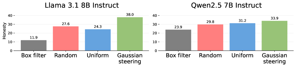
The key experimental test is an equal-budget comparison: normalize schedules to the same stated total magnitude, then vary their shape. This reduces the chance that a multi-layer method wins merely because it applies a larger summed intervention, although downstream transformations can still make equal input budgets have unequal effects.

Bar chart comparing four depth schedule strategies at equal total energy on Llama 3.1 8B Instruct and Qwen 2.5 7B Instruct. Gaussian steering achieves the highest honesty scores (38.0 and 33.9), followed by uniform (24.3 and 31.2), random (27.6 and 29.8), and box filter (11.9 and 23.9). — Equal-budget comparison of depth schedules on two models. With the same total steering energy, the Gaussian schedule consistently outperforms uniform, random, and box-filter allocations. From Góral et al., *Depth-Wise Activation Steering for Honest Language Models*. [4]

In the reported comparisons, a Gaussian schedule outperforms box, random, and uniform allocations. It reaches 38.0 on the study's honesty metric for Llama 3.1 8B, compared with 24.3 for uniform allocation, and 33.9 versus 31.2 for Qwen 2.5 7B. These results show that placement matters on the tested tasks, not only the total intervention norm.A smooth schedule may avoid sharp layer-to-layer changes, but that explanation remains a hypothesis. The comparison establishes performance differences between schedules, not why the Gaussian works.

Across seven models (spanning Llama, Qwen, and Mistral families), the Gaussian schedule improved honesty over single-layer baselines in six of seven cases. The one exception was a model where single-layer steering already worked well.

Pause and think: Why does spreading help?

Consider what happens when you add a large steering vector at a single layer. The perturbation hits the residual stream all at once, and every subsequent layer must process activations that may be far from anything seen during training. Now consider the same total perturbation spread across 10 layers: each individual nudge is small enough that subsequent layers can accommodate it without being pushed out of distribution.

One hypothesis is that several small writes cause less distribution shift at any one layer than a single large write. The numerical-integration analogy is suggestive, but “distance from the learned manifold” was not established by the schedule comparison and would require its own measurement.

If $\sigma$ becomes much larger than the model depth, the schedule approaches a uniform allocation. The reported table suggests a centered Gaussian works better on those two evaluations, but it does not determine how every intermediate width or model will rank. Test the hypothesis with a validation sweep rather than treating the ordering as architectural law.

Three Regimes Across Depth

Dang and Ngo (2026) examine one possible explanation by measuring class projections across depth [5].

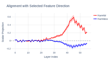
They compute the scalar projection of each class's mean activation (e.g., harmful vs. harmless) onto the steering direction at every layer. The result reveals three distinct regimes:

Line plot showing scalar projections of harmful (red) and harmless (blue) class means onto the steering direction across layers in Qwen 2.5 7B Instruct. In early layers (0-15), both projections hover near zero. In middle layers (20-40), the harmful projection rises sharply while harmless stays near zero, creating clear separation. In late layers (45+), the harmful projection drops and the gap narrows. — Class projections onto the steering direction across depth in Qwen 2.5 7B Instruct. The harmful and harmless classes separate clearly only in middle layers, with early layers showing no discrimination and late layers showing reduced separation. From Dang and Ngo, *Selective Steering*. [6]

Early layers (roughly 0-15): Both classes project near zero onto the measured direction. That direction does not separate the labels at this depth, so adding it here lacks the evidence available in middle layers. The concept could still be encoded in another form.

Middle layers (roughly 20-40): The classes separate sharply. Harmful examples project positively onto the steering direction; harmless examples project near zero or negatively. This is the discriminative zone where the concept is most clearly represented and where steering can most precisely shift behavior.

Late layers (roughly 45+ in the plotted model): Separation along this direction diminishes. This may reflect a shift toward output-specific computation, but the projection alone does not show that the model has “committed” or that the concept is absent in another form.The layer ranges come from particular models and directions. Other architectures, concepts, or extraction methods may not show the same three regimes.

The profile motivates concentrating interventions where the measured direction separates the classes. It does not by itself explain why a Gaussian schedule wins: smoothness, accumulated effects, and distribution shift are alternative mechanisms that need separate tests.

Principled Layer Selection

The three-regime picture suggests a more targeted approach: steer only at discriminative layers, and skip the rest entirely.

Dang and Ngo (2026) use an opposite-sign criterion [7]. At each layer $k$ , they project the positive and negative class means onto the steering direction and select layers where the two scalar projections have opposite signs. This is a conservative, origin-dependent selection rule. Two classes can still be well separated when both projections have the same sign, so the criterion should not be confused with a general definition of discriminability.

Layers where both classes project in the same direction, or where projections are near zero, are skipped. Steering at these layers would push both classes in the same direction without differentially affecting the target behavior.

The method also addresses norm preservation. Residual-stream norms vary across depth, so the same absolute vector is a small relative perturbation at a high-norm layer and a large one at a low-norm layer. Normalizing the intervention makes layer comparisons less confounded by this scale difference.

Dang and Ngo replace vector addition with a rotation in the plane spanned by the activation and steering direction. This preserves the Euclidean norm at the intervention site, removing one scale confound.Norm preservation does not eliminate every normalization interaction. RMSNorm depends directly on the norm, while LayerNorm also depends on the coordinate mean; a rotation can preserve the former and change the latter. Downstream nonlinear effects still require measurement.

The combination of selective layer choice and norm-preserving intervention yields large improvements: a 5.5x improvement in steering effectiveness over uniform multi-layer steering on Qwen 2.5 7B, while maintaining lower perplexity (less coherence degradation) than competing methods.

Pause and think: When would fixed schedules beat data-driven selection?

Principled layer selection requires computing class projections from labeled data, you need examples of the positive and negative class to determine which layers are discriminative. This is straightforward when steering for a well-defined binary concept like honesty or harmfulness, where labeled examples are readily available.

But what about concepts that are hard to label? Consider steering for "creativity" or "nuanced reasoning." These concepts may not decompose neatly into two classes, making it difficult to compute discriminative projections. In such cases, a Gaussian schedule requires only a center layer (findable through a simple validation sweep) and makes no assumptions about class structure. Similarly, when you have very few labeled examples, the projection estimates may be noisy enough that the simpler Gaussian is more robust.

There is a general pattern here: more data and clearer concept definitions favor more sophisticated methods, while data scarcity and concept ambiguity favor simpler schedules with fewer parameters.

Learned Layer Weights

Both Gaussian schedules and selective steering impose a fixed structure on the depth schedule: either a mathematical form or a binary include/exclude decision. Hegazy et al. (2025) take the next step: learn the per-layer weights from data [8].

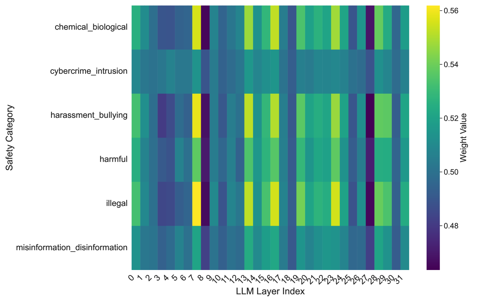
They train a small MLP controller that takes a prompt as input and outputs a weight $\alpha_k$ for each layer. The controller is trained to optimize a safety objective while keeping the model's general capabilities intact.The controller is tiny relative to the model it steers. For Llama 3.1 8B with 32 layers, it outputs 32 weights. The training uses a standard safety dataset with harmful and harmless examples, optimizing the weights to maximize the contrast between safe and unsafe completions.

The learned controller assigns different depth profiles to different labeled categories.

Heatmap showing learned controller weights across layers for six safety categories in Llama 3.1 8B. Chemical/biological content shows stronger weights in early-middle layers. Cybercrime peaks in middle layers. Harassment, harmful content, and illegal activity show varying patterns. Misinformation peaks in later layers. The weight patterns are visually distinct across categories. — Learned per-layer steering weights for different safety categories in Llama 3.1 8B. Each category induces a distinct weight pattern across depth, reflecting where each concept is most strongly encoded. From Hegazy et al., *Guiding Giants*. [9]

In the reported controller, chemical/biological examples receive more early-to-middle-layer weight, while cybercrime peaks nearer the middle and other categories have broader profiles. These are intervention policies learned for the objective, not direct maps of where each concept is represented.

Because the controller takes the prompt as input, it can produce different schedules for different examples. The observed category-level profiles are consistent with such adaptation; determining what prompt features drive the weights requires probing the controller itself.

Steering as Control

There is a deeper conceptual frame for thinking about multi-layer steering. Nguyen et al. (2025) observe that standard steering is equivalent to proportional control (the P in PID control) [10]. You measure the deviation from desired behavior (the steering vector), multiply by a gain ( $\alpha$ ), and apply the correction. One shot, open loop.

In classical control, integral and derivative terms can address steady-state error and oscillation under suitable system assumptions. The transformer analogy treats changes in alignment across layers as a trajectory, but a feed-forward network is not automatically a classical dynamical plant with the same guarantees.

Nguyen et al. implement this by treating the forward pass as a dynamical system. At each layer, a PID controller measures the current activation's alignment with the target direction and computes a correction that accounts for the cumulative effect of past interventions (I) and the rate of change (D). The controller adjusts the steering magnitude at each layer based on how much the previous layers' corrections have already shifted the model.The PID framing is appealing because it provides a principled answer to 'how much steering at each layer?' that adapts online during the forward pass rather than being fixed in advance. However, the feedback signal (projection onto the steering direction) is noisy and the 'dynamics' of a neural network forward pass are quite different from classical control systems, so the analogy should not be taken too literally.

On the reported TruthfulQA evaluation, the PID-style controller outperforms the tested single-layer and uniform baselines. Ablations of the terms are needed to support the proposed overcorrection and drift explanations; the control analogy alone does not establish them.

This framing connects multi-layer steering to a broader principle: the forward pass of a transformer is a sequential process, and interventions on sequential processes benefit from feedback and adaptation, not just feedforward injection.

Pause and think: Connecting the methods

We have now seen four approaches to multi-layer steering. Consider placing them on a spectrum from simplest to most flexible:

Gaussian schedule, fixed mathematical form, two parameters ( $\mu$ , $\sigma$ ), no data beyond a validation sweep
Selective steering, data-driven binary decisions per layer, requires labeled class examples, norm-preserving
PID controller, adaptive during the forward pass, requires tuning three gains (P, I, D), feedback-based
Learned controller, fully data-driven per-layer weights, concept-specific and input-adaptive, requires training

As we move along the spectrum, the methods gain flexibility but require more data and computation. The Gaussian schedule is a reasonable default when you have limited resources. Selective steering suits well-defined binary concepts with labeled examples. The PID approach offers online adaptation without training. Learned controllers provide maximum flexibility when training data and compute are available.

Which approach would you choose for steering a safety-critical deployment where labeled data is abundant? What about a research setting where you are exploring a novel, loosely-defined concept?

Limitations

Multi-layer steering improves on single-layer approaches, but several open problems remain.

Same vector across all layers. All methods discussed here use the same steering vector $\mathbf{v}$ at every layer, varying only the scalar weight $\alpha_k$ . But concept directions may rotate across depth, the direction that encodes "honesty" at layer 10 may not be the same direction at layer 30. Per-layer vector adaptation remains largely unexplored.

Interaction with other steering types. Multi-layer distribution has been studied primarily for addition steering. How it interacts with affine steering (which includes a re-centering step) or ablation steering (which projects out a direction) is unknown. The re-centering in affine steering, for instance, is calibrated for single-layer intervention, distributing it across layers would require rethinking the affine correction.

Narrow evaluation. Most results focus on honesty, harmlessness, or similar binary safety benchmarks. Whether multi-layer steering improves outcomes for more subtle behavioral dimensions (helpfulness, creativity, nuanced reasoning) is an open question.

No unified theory. We have empirical evidence that Gaussian schedules work, that discriminative layers matter, and that learned weights vary by concept. But there is no theoretical framework explaining why a particular depth distribution is optimal, or predicting the best schedule from model architecture alone.

Looking Ahead

Multi-layer steering shifts the question from “which layer?” to “how much at each layer?” That turns a discrete site choice into a schedule-design problem, with fixed, data-driven, and adaptive approaches that can be compared under matched intervention budgets.

Interpretability-Guided Training changes the time axis as well as the depth axis. Instead of adding a schedule only during deployment, it asks whether directions and probes can reshape the examples, activations, or rewards used for training.

A later block develops richer intervention units. Sparse autoencoders and transcoders decompose activations into interpretable features, enabling control at the feature level rather than only along a supervised direction.