Probing Classifiers

From Predictions to Representations

The logit lens and tuned lens project intermediate states to vocabulary space, answering "what would the model predict at this layer?" Probing classifiers ask a different question: "what information is encoded in the representations at this layer?"

A probing classifier is a simple model, typically linear, trained to predict a linguistic or semantic property from the internal activations at a given layer:

\hat{y} = \text{Probe}(\mathbf{h}_\ell) = \sigma(W_p \mathbf{h}_\ell + \mathbf{b}_p)

If a linear probe achieves high accuracy, the information is present and linearly accessible in the representations. The probe's simplicity is deliberate: a powerful nonlinear probe might learn the property itself rather than detecting it in the representations.

Probing Classifier: A probing classifier is a simple model (typically linear) trained to predict a linguistic or semantic property $y$ from the internal activations $\mathbf{h}_\ell$ of a neural network at layer $\ell$ . High probe accuracy indicates the property is encoded in the representations. The probe's simplicity ensures that a successful readout reflects information in the representations, not computation performed by the probe itself.

Why restrict probes to be linear? The restriction connects directly to the linear representation hypothesis: if features are represented as linear directions in activation space, then a linear probe is exactly the right tool to detect them. A nonlinear probe might succeed even on random representations by performing substantial computation of its own, rendering the results uninterpretable.The question of probe complexity is a recurring theme in the probing literature. If a two-layer MLP probe achieves higher accuracy than a linear probe, does that mean the information is encoded nonlinearly? Or does it mean the MLP probe is partially computing the property rather than merely reading it? There is no consensus answer, which is one reason the field has gravitated toward linear probes as the default.

Structural Probes: Beyond Labels

Hewitt and Manning (2019) pushed probing beyond simple classification by introducing structural probes [1]. Instead of asking "is this token a noun?", they asked: "does the geometry of the representations encode the entire syntax tree?"

The key idea: find a linear transformation $B$ under which the squared L2 distance between word representations encodes parse tree distance:

d_B(\mathbf{h}_i, \mathbf{h}_j)^2 = (B(\mathbf{h}_i - \mathbf{h}_j))^T B(\mathbf{h}_i - \mathbf{h}_j) \approx \text{tree\_distance}(i, j)

Gold parse trees (black arcs) compared with trees recovered by the structural probe from BERT-large layer 16 (blue), ELMo layer 1 (red), and a non-contextual baseline (purple). BERT's recovered tree closely matches the gold parse tree, while the baseline fails to capture long-range syntactic structure. — Gold parse trees (black) compared with trees recovered by the structural probe from BERT-large layer 16 (blue), ELMo layer 1 (red), and a non-contextual baseline (purple). The probe finds a linear transformation under which distances between word representations approximate parse tree distances, allowing full tree recovery. From Hewitt and Manning, *A Structural Probe for Finding Syntax in Word Representations*.[2]

Their results showed that syntax trees are embedded in a linear subspace of BERT representations. Different layers encode different syntactic details: earlier layers capture local structure, later layers capture longer-range dependencies. The structural probe levels off with increasing rank, indicating a lower-dimensional syntactic subspace within the full representation.

Probes can detect not just labels but relational structure in representations. The promise is tantalizing: we can read rich, structured information directly from how the model represents language internally.

Sparse Probing: Constraining What the Probe Can Access

Standard linear probes use all neurons in a layer. But if we want to understand how information is organized, a more revealing question is: how many neurons does the probe actually need?

k-sparse probing constrains the probe to use at most $k$ neurons [3]. Rather than fitting a weight vector over all $d$ neurons in a layer, the probe selects the $k$ most informative neurons and fits weights only on those. This is a hard L0 constraint (exactly $k$ nonzero weights), not L1 regularization.

The results reveal how features are organized across neurons:

At $k = 1$ , middle-layer neurons in large models can individually classify features like "is Python code," specific natural languages, and data distributions with high accuracy. These are monosemantic neurons: single neurons dedicated to single concepts.
In early layers, $k = 1$ performance is poor. Features like "contains a digit" require $k = 5$ or more neurons. The feature is distributed across multiple polysemantic neurons, each of which individually responds to many unrelated inputs. This is precisely the pattern predicted by superposition.
Sparsity increases with model scale. Across the Pythia model family (70M to 6.9B parameters), larger models encode features more sparsely on average: a feature that requires $k = 8$ neurons in a small model may need only $k = 2$ in a large model. As capacity grows, models transition from cramming features into shared neurons (superposition) to allocating dedicated neurons (monosemantic representation).

A rotation baseline confirms these findings are not artifacts of the probing method. Randomly rotating the activation space and repeating $k = 1$ probing destroys performance, confirming that the standard neuron basis is privileged: features genuinely align with individual neurons, rather than being extractable from any arbitrary basis.Sparse probing connects probing to the superposition research program. If features are in superposition (more features than neurons, encoded as sparse combinations), then a sparse probe should reveal this: features in superposition require higher $k$ , while monosemantic features need only $k = 1$ . The finding that early layers require higher $k$ and later layers less is direct evidence for the superposition hypothesis in real models.

Sparse probing also sharpens the probe complexity debate. The concern with standard probes is that a powerful probe might learn the property rather than detect it. Sparse probes address this from a different angle: even if the probe is linear, constraining it to use very few neurons limits what it can learn. A $k = 1$ probe that achieves 85% accuracy on a feature is strong evidence that the feature is genuinely encoded in that neuron, not computed by the probe.

But probe accuracy, whether sparse or dense, still faces a more fundamental challenge.

The Probing Critique: Correlation vs. Causation

High probe accuracy tells us information exists in the representations. It does not tell us the model uses that information. This is the correlation-vs-causation gap at the heart of the probing debate.

MDL Probing: Measuring Effort, Not Accuracy

Voita and Titov (2020) demonstrated that probe accuracy alone is an inadequate metric [4]. Their key finding is striking: a probe can achieve similar accuracy on pretrained representations and random representations. If a probe can decode a property from random vectors, that property is not meaningfully "encoded" in any useful sense. The probe is simply powerful enough to memorize the mapping.

Minimum Description Length (MDL) probing reframes the question. Instead of asking "can a probe predict this property?", ask "how much effort does the probe need?"

Better representations require simpler probes (lower description length). Think of it as compression: good representations compress the labels more, requiring less effort to decode them. A representation where part-of-speech can be read off with a simple weight vector encodes POS more accessibly than one where the probe needs thousands of training examples and a high-rank weight matrix to decode the same labels.

MDL probing is more informative than accuracy alone. It distinguishes between representations where information is readily available (low MDL) and representations where the probe must do significant computation (high MDL). But MDL is still a correlational measure. It tells us how easily accessible a property is, not whether the model actually accesses it.

Amnesic Probing: The Bridge to Causation

Elazar et al. (2021) took the crucial next step [5]. Instead of asking "can we decode property $Z$ ?", they asked: "what happens to task performance if we remove property $Z$ ?"

Their method uses Iterative Null-Space Projection (INLP) to project out a property from the representations, then measures the behavioral impact on the model's downstream task. If removing a property hurts performance, the model relied on it. If removing it has no effect, the model encoded the property but did not use it.

The key finding is a direct challenge to the probing paradigm: conventional probing performance is not correlated with task importance. Consider this scenario:

A linear probe detects part-of-speech with 95% accuracy at layer 6.
But removing POS information from layer 6 does not hurt language modeling performance.
The information is there but the model does not rely on it.

Conventional probe accuracy told us the wrong story. A property may be easily decodable but irrelevant -- the model encodes it as a byproduct, not as a functional component. Or a property may be hard to decode but essential -- the model uses it in a way that a linear probe cannot easily extract.

This disconnect is the most important lesson of the probing literature [6]. Probes detect correlations, not causes. Random baselines are essential for context. And the most sophisticated probing method (amnesic probing) points beyond probing altogether, toward the causal intervention methods that can definitively answer what the model relies on.

Pause and think: Probes and causation

A probe achieves 95% accuracy at detecting part-of-speech from layer 6 activations. Does the model "know" POS? Does it "use" POS? How would you test the difference?

The model "knows" POS in the sense that the information is linearly decodable from its representations. But "knowing" and "using" are different. To test whether the model uses POS, you would need an intervention: remove POS information (via amnesic probing or activation patching) and measure whether downstream task performance degrades. If it does, POS is causally relevant. If it does not, POS is a byproduct -- encoded but not relied upon.

Attention Pattern Visualization

A related observational tool is the most intuitive: look at where attention heads direct their focus. We examined attention patterns briefly in the context of direct logit attribution. Here we see them applied to real model data.

Consider GPT-2 Small processing a repeated sequence: "The cat sat on the mat. The cat sat on the." Two heads display distinctive patterns:

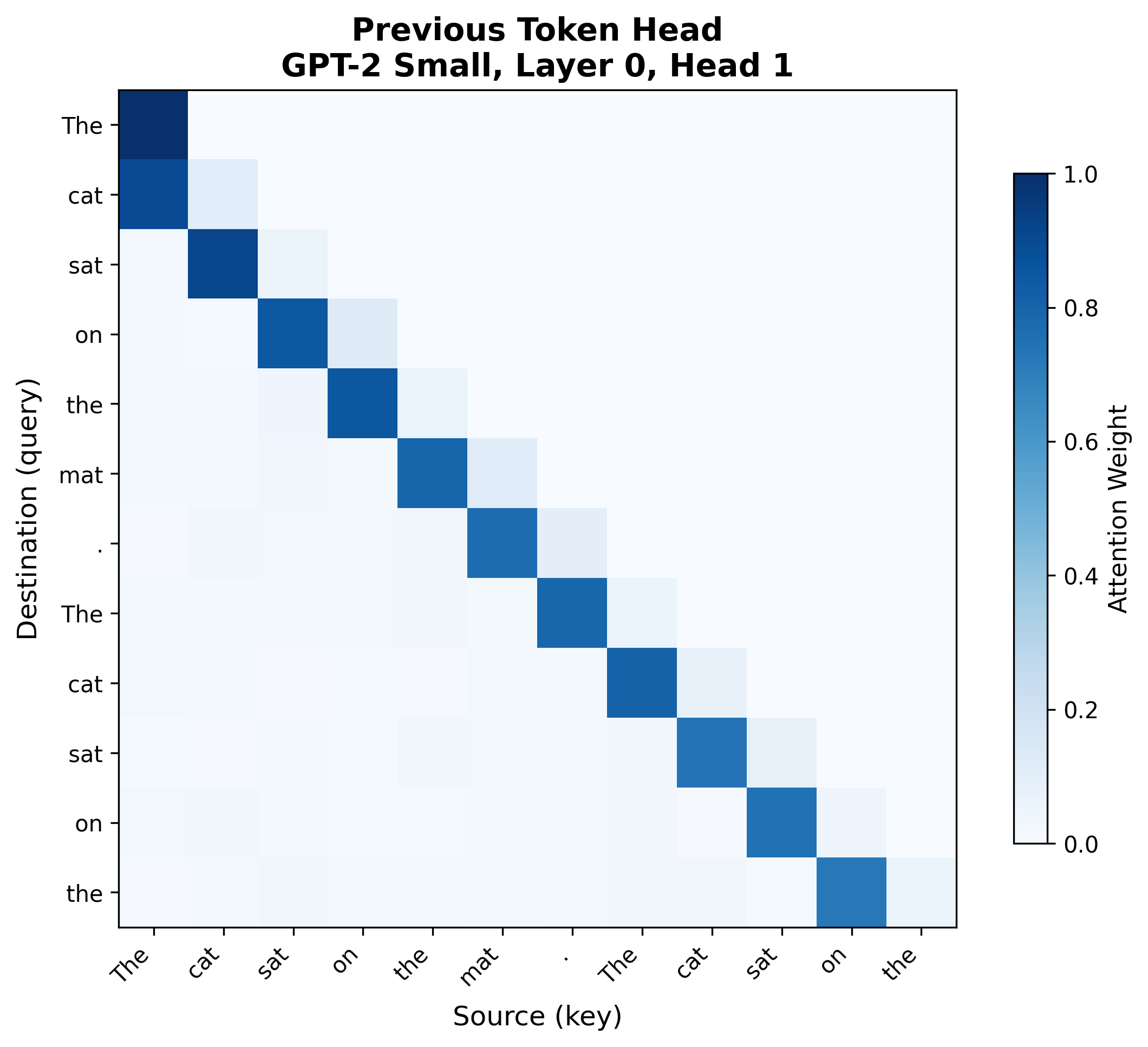
Previous token head attention pattern showing a clear diagonal line where each position attends to the position immediately before it. — Figure 2: Previous token head (Layer 0, Head 1) in GPT-2 Small. The strong diagonal pattern shows each token attending to its immediate predecessor.

Induction head attention pattern showing off-diagonal attention where repeated tokens attend to tokens that followed their first occurrence. — Figure 3: Induction head (Layer 5, Head 1) in GPT-2 Small. In the second half of the sequence, attention jumps to specific positions in the first half, attending to tokens that followed the first occurrence of each repeated token.

The left pattern is a previous token head (Layer 0, Head 1): a clean diagonal where each position attends to the position immediately before it. This head implements the first step of the induction circuit, writing "my predecessor was token X" into each position's residual stream.

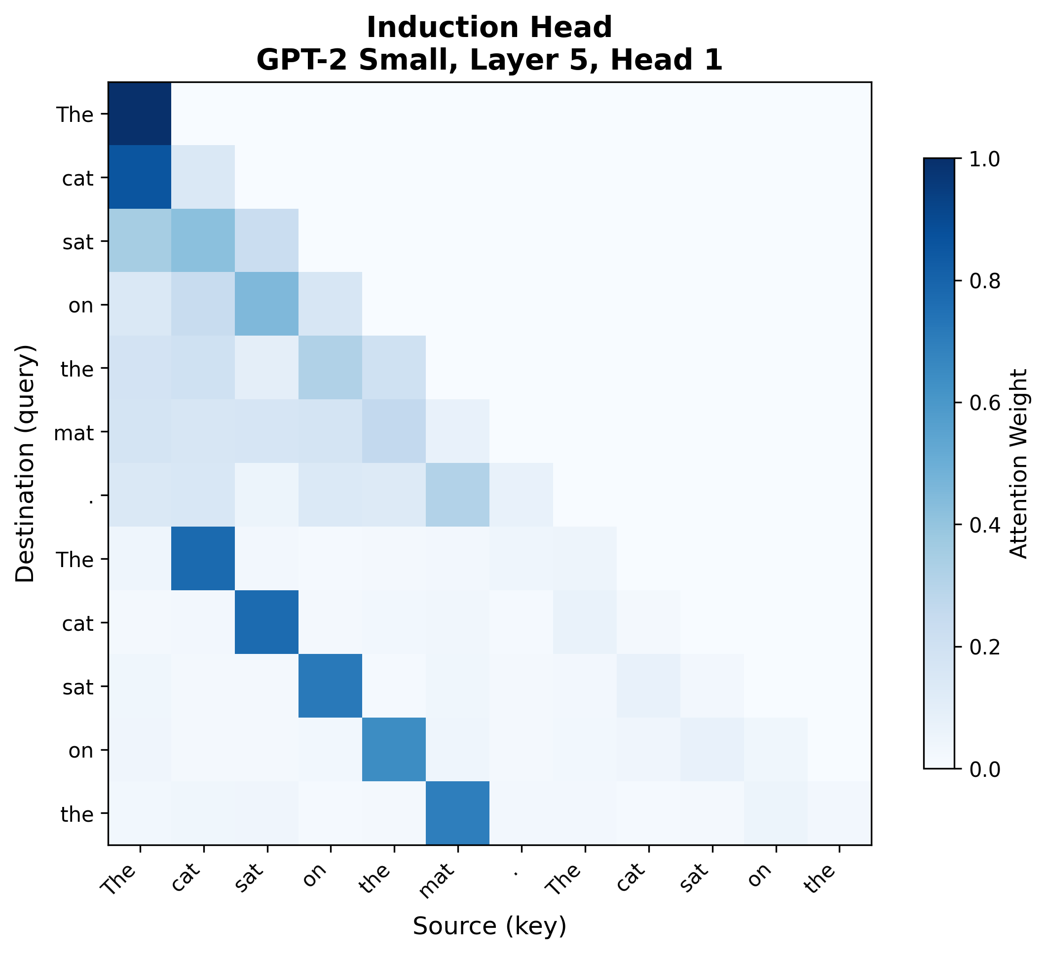
The right pattern is an induction head (Layer 5, Head 1): in the second half of the repeated sequence, attention jumps to specific positions in the first half. The second "The" attends to " cat" (the token after the first "The"). This head implements the second step: querying "who has predecessor equal to my current token?" and copying that position's token to the output.These attention patterns are from actual GPT-2 Small runs in TransformerLens, not idealized illustrations. Real attention patterns are messier than textbook diagrams -- notice that the previous token head has some diffuse attention beyond the strict diagonal, and the induction head has background attention to various positions. The diagnostic patterns are strong enough to identify the head types, but interpreting attention requires looking at the dominant structure, not expecting perfect textbook examples.

These visualizations let us see the two-step mechanism we studied theoretically. But attention patterns reveal only where a head looks, not what it does with the information. The attention pattern comes from the QK circuit. What information gets moved comes from the OV circuit. Two heads with identical attention patterns can have completely different effects on the output.

The Key Limitation: Observation Cannot Establish Causation

Probing classifiers detect what information is linearly decodable from representations. They can reveal rich structure, from part-of-speech labels to syntax trees. But probe accuracy is not correlated with task importance. Information can be encoded yet unused. Attention patterns show where heads look, but not what information the head moves or whether the attended information matters downstream.

None of these tools establish whether the detected information is causally necessary for the model's behavior. A probe detects syntax at layer 6, but does the model use syntax at layer 6? A head attends to the previous token, but does that attention matter for the output?

All observational tools establish correlations: the information co-occurs with the activations. To establish causation, we need a different kind of experiment, one where we intervene on the model's internals and observe changes in behavior. If we change an intermediate activation and observe a change in the model's output, we have causal evidence.

This is the shift from observation to causation, and it is the subject of the next articles. Activation patching replaces one component's activation with an activation from a different input and measures the effect on predictions. Path patching traces the causal flow through specific pathways in the computational graph. These tools complete the methodological toolkit, moving us from "what exists?" to "what matters?"

Observation reveals what exists. Only intervention reveals what matters. We can look inside the model. But looking is not the same as proving.